 |
The AHA Model
Revision: 17463
Reference implementation 04 (HEDG02_04)
|
|
The AHA Model
Revision: 17463
Reference implementation 04 (HEDG02_04)
|
This is a large scale simulation model (under development) that implements a general decision-making architecture in evolutionary agents. Each agent is programmed as a whole virtual organism including the genome, rudimentary physiology, the hormonal system, a cognitive architecture and behavioural repertoire. They "live" in a stochastic spatially explicit virtual environment with physical gradients, predators and prey. The primary aim of the whole modelling machinery is to understand the evolution of decision making mechanisms, personality, emotion and behavioural plasticity within a realistic ecological framework. An object-oriented approach coupled with a highly modular design not only allows to cope with increasing layers of complexity inherent in such a model system but also provides a framework for the system generalizability to a wide variety of systems. We also use a "physical-machine-like" implementation philosophy and a coding standard integrating the source code with parallel detailed documentation that increases understandability, replicability and reusability of this model system.
The cognitive architecture of the organism is based on a set of motivational (emotional) systems that serves as a common currency for decision making. Then, the decision making is based on predictive assessment of external and internal stimuli as well as the agent's own motivational (emotional) state. The agent makes a subjective assessment and selects, from the available repertoire, the behaviour that would reduce the expected motivational (emotional) arousal. Thus, decision making is based on predicting one's own internal state. As such, the decision-making architecture integrates motivation, emotion, and a very simplistic model of consciousness.
The purpose of the AHA model is to investigate a general framework for modelling proximate decision-making and behavior. From this we will investigate adaptive goal-directed behaviour that is both guided by the external environment and still is endogeneously generated.
Other research topics include individual differences, personality as well as consequences of emotion and personality to population ecology.
We think that understanding and modelling complex adaptive behaviour requires both extraneous (environmental) factors and stimuli as well as endogeneous mechanisms that produce the behaviour. Explicit proximate representation of the motivation and emotion systems, self-prediction can be an important component in linking environment, genes, physiology, behavior, personality and consciousness.
Fortran is used due to its simplicity and efficiency. For example, check out this paper: Why physicists still use Fortran?.
Main features of modern Fortran that are used in the AHA model code are briefly outlined in the README_NF .
This is the model version information parsed from the main Subversion repository https://svn.uib.no/aha-fortran or Bitbucket Mercurial-based repository https://bitbucket.org/ahaproject/hedg2_01 (the latter is currently used just as a mirror of the Subversion branch).
$Id: m_common.f90 9552 2020-06-06 07:26:50Z sbu062 $
Version information is also saved as two variables that can be passed to the logger (see commondata::logger_init()) and outputs and file names:
A "Getting Started" introduction is available in the README.md file.
The Modelling framework is composed of two separate components:
Building and running the mode is based on the GNU Make system.
FC variable, e.g. DEBUG variable. See Makefile for build configuration. To get more information on GNU Make see AHA Modelling Tools Manual, Using Microsoft Visual Studio and Using Code::Blocks IDE.
The model makes use of several environment variables to control certain global aspects of the execution. These variables have the AHA_ prefix and are listed below.
AHA_DEBUG=TRUE sets the debug mode;AHA_SCREEN=YES sets logger to write to the standard output in addition to the log file;AHA_DEBUG_PLOTS=YES enables generation of debug plots;AHA_ZIP_FILES=YES enables background compression of big output data files;AHA_CHECK_EXTERNALS=NO disables checking for external executable modules (this is a workaround against Intel Fortran compiler bug).They are described in details in the commondata::system_init() section. Setting the environment variable on different platforms: Linux/Unix:
Windows:
Checking if the environment variable is set and what is it value On Unix/Linux:
On Windows
To check if any of the above environment variables are set is easy on Linux:
The protected global variable IS_DEBUG (commondata::is_debug) sets up the debug mode of execution. The debug mode results in huge amount of output and logs that significantly slows down execution. Debug mode can be set using the environment variable AHA_DEBUG=1, AHA_DEBUG=YES or AHA_DEBUG=TRUE. Debug mode can also be set by setting the runtime command line parameter to DEBUG, DEBUG=1, DEBUG=YES or DEBUG=TRUE to the model executable, e.g.
This runtime command line parameter is automatically set if the model is started using the DEBUG variable for the GNU Make:
Build Note also that DEBUG with make build command
will build the executable for the model in the debug mode also. All compiler optimisations are turned off (-O0), debugger symbols (-g) and tracebacks are enabled, various compiler error checking options and warnings are also enabled, along with extended runtime checks.
Notably, the Intel Fortran compiler enables initialisation of variables with the signalling NaNs (-init=snan). Any operations on non-initialised variable(s) would then result in the runtime crash with traceback, making it easier to catch non-initialised variables.
Normal build without setting DEBUG, in contrast, enables various compiler optimisations making the executable run faster.
Notably, with the Intel Fortran compiler, the model is built with automatic parallelisation (-parallel), so whole array operations, do concurrent and pure and elemental functions are run in the multi-threaded mode whenever the compiler is "sure" that these operations can be safely performed. See the Makefile for specific compiler and debugging options and the GNU make for a general overview of the system. A overview of Intel Fortran parallel processing options can be found here and here.
Combining the shell environment variable AHA_DEBUG and the DEBUG make variable allows to control how the model executable is build and run. For example, building it in non-debug mode, i.e. with all the optimisations for fast (and possibly multi-threaded) execution:
can be combined with running the model in the debug mode:
In such a case, the model is built and executed in the "fast" optimised and possibly multi-threaded mode, but still prints all the numerous debugging outputs into the logger.
The system initialisation procedure commondata::system_init() and commondata::logger_init() provide more details on initialisation and logging.
At the start of the simulation, the program creates an empty lock file defined by commondata::lock_file. The lock file is created at the end of commondata::system_init() and and is deleted by the procedure commondata::system_halt().
The lock file indicates that the simulation is (still) running and could be used by various scripts, cron jobs etc to make sure the simulation is finished. For example, a script can check from time to time if the lock file exists and if not, issue a command to zip all data outputs and transfer them to a remote analysis server.
The stop file is an effective method to terminate the simulation at any generation and avoiding any destructive consequences that would be caused, for example, by using the Ctrl+C keypress or kill command. Thus, the stop file is a signalling file.
The name of the stop file is defined by the parameter commondata::stop_file. This file is checked upon each new generation of the Genetic Algorithm in the_evolution::generations_loop_ga() (CHECK_STOP_FILE block). If this file is found, simulation will not proceed to the next generation and will just stop as if it were the last generation. All the data are saved as normal.
touch stop_simulation_running.lock. On Windows, these two command can be used for the same purpose: type nul > stop_simulation_running.lock or copy NUL stop_simulation_running.lock. The lock file is deleted by make cleandata command. Note also that once the stop file is created in the model running directory, actual stop is not immediate: it will be executed only at the next generation, the currently running generation is completed to its end as normal.Data could be output from the model. The standard format for data output is CSV. Its advantage is that it is based on plain text and is human readable nut can be easily imported into spreadsheets and statistical packages. The most straightforward use for CSV is for vector-based data and two-dimensional matrices, including sets of vectors (e.g. 'variables'/columns with 'observations'/rows).
CSV output is based on the CSV_IO module in HEDTOOLS. There is also an object oriented wrapper for CSV_IO: file_io.
The model also includes a few standardised CSV output procedures for saving various characteristics for a whole population of agents:
Additionally, the genetic algorithm subroutine the_evolution::generations_loop_ga() implements a sub-procedure
The following procedures output the properties of the the_environment at a particular time step:
The model includes several descriptors that can be used for descriptive notes on the model.
These descriptors can appear in the model logger output and form parts of the output data files.
In particular, because the Model Abstract is stored in a separate text file, it can contain dynamically updated information, such as the latest version control message log output. Subversion and Mercurial commit hooks can be used to implement such a functionality.
To append version information (Subversion) to the Model Abstract file manually do this:
Using a consistent coding style increases the readability and understandability of the program. It is also easier to search and locate specific parts. For example, using specific rules for version control commit messages make it easier to find specific changes by using regular expression syntax. The coding rules for the AHA model are relatively light.
intent declared for all subroutines and functions.SPATIAL and SPATIAL_MOVING) use position to set spatial position and location to get it.create method is used to create and initialise an empty object (e.g. SPATIAL with missing coordinates), should not take other parameters and must be elemental (so cannot include calls to random);make or build method is used to create a working object with random initialisation etc.See the AHA Modelling Tools Manual for more details (http://ahamodel.uib.no/doc/HEDTOOLS.pdf).
The README_NF provides a brief outline of the main features of modern Fortran (F2003/2008) that are used in the model code.
HIDE_IN_BODY_DOCS is NO.###: this\%reprfact_decrement_testosteronenot
`this\%reprfact_decrement_testosterone`or
this%reprfact_decrement_testosteroneor still
`this%reprfact_decrement_testosterone`as the percent sign disappears in the parsed output.
     !! values resulting from executing this behaviour (`reproduce::do_this()`
     !! = the_neurobio::reproduce_do_this() method). This is repeated for
This makes them appear as cross-links in the parsed document. !> Calculate the Euclidean distance between two spatial objects.
!! See `the_environment::spatial_distance_3d()`
procedure, public :: distance => spatial_distance_3dcontains) is using the hanging :: notation: !! The subjective capture probabilityis calculated by the sub-function
!! `::subjective_capture_prob()`.!> @subsubsection aha_buildblocks_genome_genome Individual genomeThey can be referred to in the documentation text using the tag like this:
!> @ref aha_buildblocks_individual "The individual agent" is also ...
type definitions to delimiter outer procedure interfaces.There are many possible quirks and caveats with the real type (float point) calculations on the computer. The rules of float point computations deviate from the basic arithmetic. The main issue is that real type numbers are represented as bits and have finite and limited precision. Furthermore, numerical precision can deteriorate due to rounding in computations.
The precision of the float point number representation in Fortran is controlled by the kind parameter (e.g. real(kind=some_number) ).
Numerical precision modes. In the AHA Model, there are two basic numerical precision modes:
Constants. There is also a useful commondata::zero constant, which sets some "minimum distinguishable non-zero" value: it is the smallest real number E such that  .
.
The smallest positive real value is defined by the commondata::tiny_srp constant. It is used in the definition of the default numerical tolerance value for high precision calculations:
Because the low tolerance based on the commondata::tiny_srp and commondata::tiny_hrp may be too small and restrictive in many cases, the second set of tolerance limits for low-precision calculations is based on the commondata::zero parameter:
epsilon in most cases.The default commondata::srp values of these parameters calculated on an x86_64 platform under Linux are (an example only!):
   ZERO: 1.19209290E-07
   TINY_SRP: 1.17549435E-38
   TOLERANCE_LOW_DEF_SRP: 5.87747175E-38
   TOLERANCE_HIGH_DEF_SRP: 1.19209290E-04
These constants are reported at the start of the logger output.
Real type equality. One possible quirk in float point computation involves equality comparison, e.g.
With real type data a and b, such a condition can lead to unexpected results due to finite precision and even tiny rounding errors: the numbers that are deemed equal may in fact differ by a tiny fraction leading to a == b condition being FALSE.
Instead of the exact comparison, one should test whether the absolute difference is smaller than than some predefined  tolerance value (in the simplest case):
![\[ \left | a-b \right | < \varepsilon \]](form_96.png)
The is chosen based on the nature of the data and the computational algorithm.
The AHA Model framework includes a specific function for testing approximate equality of two reals: commondata::float_equal(). With this function, correct comparison is:
There is also a user defined operator "float equality" .feq. that works as the commondata::float_equal() function, but uses a fixed default epsilon equal to the default tolerance commondata::tolerance_low_def_srp (or commondata::tolerance_low_def_hrp for high precision). Its benefit is that the usage almost coincides with the == (.eq.) operator usage:
See the backend procedures commondata::float_equal_srp_operator() and commondata::float_equal_hrp_operator() for details. Another similar operator is "approximate equality" .approx. has a much higher level of tolerance (larger error accepted)
See the backend procedures commondata::float_approx_srp_operator() and commondata::float_approx_hrp_operator() for details.
There is also a function for testing if a real value is approximately equal to zero: commondata::is_near_zero():
When a variable is created but not yet initialised, its value is "undefined". However, it can take some haphazard values depending on the compiler and the platform. There are special "initialisation" constants defined in commondata that set "missing" or "undefined" variable status: commondata::missing (real) and commondata::unknown (integer). By default, they are set to an unusual negative number -9999, so that any bugs are clearly exposed if a variable inadvertently uses such an "undefined" value.
The model in many cases makes use of nonparametric relationships between parameters. This is based on the linear and non-linear interpolation procedures implemented in HEDTOOLS: Interpolation routines
Instead of defining specific function equation linking, say, parameters X and Y: Y=f(X), the relationship is defined by an explicit grid of X and Y values without specifying any equation.
In the simplest two-dimensional case, such a grid is defined by two parameter arrays, for the abscissa and the ordinate of the nonparametric function. Any values of this function can then be calculated based on a nonlinear interpolation. This makes it very easy to specify various patterns of relationships even when exact function is unknown or not feasible.
An example of such a nonparametric function is the_neurobio::gos_global::gos_find().
AHA/BEAST Resources:
Tools web resources:
The environment is a full 3D space, that is has the class the_environment::spatial as the elementary base primitive. The the_environment::spatial is a single object that has X, Y and Z (depth) coordinates. the_environment::spatial_moving extends the basic the_environment::spatial object by allowing it to move. Furthermore, the_environment::spatial_moving includes a history stack that records the latest history of such a spatial moving object. Examples of spatial moving objects can be food items (the_environment::food_item), predators (the_environment::predator), and more complex objects composed of several the_environment::spatial components like the_environment::environment.
The basic environment where the agents "live" is very simplistic in this version of the model. It is just and empty box. The box is delimited by the basic environmental container: the_environment::environment class. The the_environment::habitat class is the ecological "habitat", an extension of the basic the_environment::environment that adds various ecological characteristics and objects such as the_environment::food_resource, array of the_environment::predator objects etc.
Normally, the movement of the agent is limited to a specific the_environment::environment container with its own the_environment::habitat. All the habitats that are available for the agents are arranged into a single global public array the_environment::global_habitats_available.
The individual agent is also an extension of the the_environment::spatial class: the_environment::spatial → the_environment::spatial_moving → the_genome::individual_genome → ... → the_population::member_population.
A brief outline of the genetic architecture, defined in the_genome, is presented on this scheme.
The agent has genes (class the_genome::gene) that are arranged into chromosomes (class the_genome::chromosome). Each gene also includes an arbitrary number of additive components (see the_genome::gene).
Here is a brief outline of the chromosome structure. The chromosomal architecture allows arbitrary ploidity (however haploid is not supported, although can be easily added), i.e. agents with diploid and polyploid genomes can be implemented. Ploidity is defined by a single parameter commondata::chromosome_ploidy.
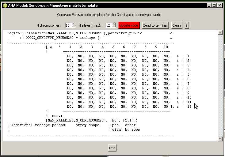
Correspondence between the genotype and the phenotype (hormones, neurobiological modules etc.) is represented by boolean Gene x Phenotype matrices. Any arbitrary structure can be implemented, many traits controlled by a single gene, many genes controlling a specific single trait.
An example of such a structure is the genetic sex determination: commondata::sex_genotype_phenotype.
There is a small utility script tools\gpmatrix.tcl that assists in automatic production of the Fortran code for such a matrix.
The the_genome::individual_genome class defines the basic higher-level component properties of the whole organism, such as sex (logical type the_genome::individual_genome::sex_is_male), genome size (the_genome::individual_genome::genome_size), individual string "name" of the agent (the_genome::individual_genome::genome_label) etc.
The the_genome::individual_genome class also includes such type-bound procedures as the_genome::individual_genome::lives() that gives the agent the "alive" status, the_genome::individual_genome::dies() for making the agent "dead". It also has linked procedures implementing genetic crossover
The individual agent has a the_environment::spatial_moving class as its base (but this class is an extension of the simple the_environment::spatial) and is then composed of several layers by class extensions.
Each of these main layers that create the individual agent is defined in separate Fortran module:
The model code benefits from Fortran intrinsic "elemental" and array-based procedures. To initialise a whole population of random agents (with full object hierarchy) use the the_population::population::init() method:
Invocation of the 'init' method calls a whole cascade of various elementary object-bound procedures that create the whole population object.
The model is based on (almost) fully proximate and localist philosophy. All objects (agents, predators, prey) can obtain information about only those objects that in proximity. No one is considered omniscient. Thus, objects can only interact locally, e.g. the agent can eat only food items that it could see, a predator could only attack agents that are visible to it etc.
The distance at which the objects can get information about each other is based on the visibility (visual range). Thus, the agents and predators are considered to be fully visual creatures that can only sense the world with their vision.
Visibility, i.e. the distance from which an object can be detected ("seen") depends on the ambient illumination at a specific depth, the area of the object, its contrast etc. Visual range is calculated for the different kinds of objects using the the_environment::visual_range() backend.
Examples of the visual range are the visibility distance of an agent the_body::condition::visibility(), food item the_environment::food_item::visibility(), and predator the_environment::predator::visibility().
Importantly, the perception of various kinds of environmental objects by the agent uses the the_environment::visual_range() calculation engine.
Furthermore, probabilities of stochastic events typically have non-linear relationships with the visual range. One example is the probability of capture of a food item by the agent. This probability is high in close proximity but strongly reduces at the distance equal to the visual range limit: the_environment::food_item::capture_probability(). Similarly, the risk that the agent is killed by a predator is highest at a small distances and significantly reduces at a distance equal to the visibility limit (i.e. the maximum distance the predator can see the agent): the_neurobio::perception::risk_pred(). A more complex procedure is implemented for the probability of successful reproduction: the_neurobio::appraisal::probability_reproduction().
The cognitive architecture of the agent is represented on the scheme below. It includes several functional units, "bundles," each representing specific motivation or emotion state.
 .
.General. The agent perceives the outer and its own inner environment, obtaining perception (signal) values. The agent also has several motivation (emotional) states, such that only one can be active at any time step of the model. Thus, the states compete for this position. The winning motivation (emotion) becomes the dominant emotional state of the agent, its Global Organismic State. This Global Organismic States of the agent determines how the agent weights different options during its decision making process and therefore determines what kind of behaviour (action) it will execute.
Perception and appraisal. The agent obtains perceptions (P) from its external and internal environments. These perceptions are fed into the Appraisal modules, separate for each of the motivation/emotion state.
Here perception signals are first fed into the neuronal response functions (based on the sigmoidal function commondata::gamma2gene()). The neuronal response function is a function of both the perception signal (P) and the genome (G) of the agent. Perception signal is also distorted by a random Gaussian error. Each neuronal response function returns the neuronal response (R) value.
The neuronal responses R for each stimulus are summed for the same motivation module to get the primary motivation values (  ) for this motivational state. These primary motivations can then be subjected to genetic or developmental (e.g. age-related) modulation, resulting in the final motivation values (
  ). Such modulation could strengthen or weaken the motivation values and therefore shift the outcome of competition between the different motivational states. In absence of modulation
  .
.
Global Organismic State. Final motivations ( ) for different motivations (emotions) are competing, so that the winning state that is characterised by the highest final motivation value becomes the dominant emotional state of the agent: its Global Organismic State at the next time step. Additionally, the final motivation value of this state becomes the GOS arousal level.
The competition mechanism is complex and dynamic. It depends on the current arousal level, such that relatively minor fluctuations in the stimuli and their associated motivation values are ignored and do not result in switching of the GOS to a different state.
Furthermore, the relative difference (surplus) that the competing motivation must have to win competition against the current state depends on the current level of GOS arousal. If the current arousal level of the agent is relatively low (motivation or emotion is weak), a competing state must exceed a relatively higher threshold to win. However, if the current arousal level is very high (high motivation or emotion), a competing state can win even if it only slightly exceeds the current arousal level. Thus, the emotional state of the agent is characterised by a degree of continuity or "inertia" and such inetria is lower the higher is the current level of arousal. The dynamic threshold mechanism for GOS competition is described in details in the_neurobio::gos_find_global_state() procedure documentation section.
Attention focus. Whenever the agent has a specific Global Organismic State, this state also affects the agent's perception. All the perception inputs that belong to motivations other than the currently dominant (i.e. the current GOS) are suppressed by attention weights. For example, if the motivation B is the GOS, all the perception values linked with Motivation A and C are suppressed. The suppression weights are proportional to the current GOS arousal of the agent.
Thus, the attention mechanism effectively filters out or "focus" the agent on the stimuli that are linked with the current dominant emotional state. Moreover, the stronger is the current GOS arousal, the stronger is such attention focusing. Attention weight mechanism is described in details in the the_neurobio::gos_attention_modulate_weights() procedure section.
Perception-to-arousal path. This process, perception → neuronal response → motivation → GOS → arousal is repeated at each time step of the model as the agent acts in (e.g. moves through) its stochastic environment. In effect, the dominant motivational and emotional state of the agent changes adapting to to the latest changes in the inner and external environment.
Self-predictive decision making. Furthermore, the same processes (and computer code procedures) are also evoked when the agent is making the decision about what behavioural action to choose at each time step.
Basically, the agent predicts what would be its perceptions and, for each of the behavioural action available, runs the same process (perception → neuronal response → motivation → GOS → arousal) and finally selects the behaviour that would result in the lowest predicted GOS arousal. Perceptions in this process are predicted from the agent's internal or local external environment ("fake" perceptions in the do_this method for each of the behaviour units). They are also subjected to attention suppression, however, attention weights are transferred from the agent's own current Global Organismic State by the_behaviour::behaviour_base::attention_transfer() method.
Thus, decision making of the agent is based on predicting one's own emotional state. The emotional arousal therefore becomes a common currency in decision making. See Predictive decision making for more details.
Goal directed behaviour. The cognitive architecture implemented in the AHA model effectively produces goal-directed behaviour in the agents. The "goal" is defined by the evolutionary process, the Genetic Algorighm. Specifically , the target "goal" is to survive, grow, accumulate energy and reproduce. The agents that do best in this respect pass their genes into the next generation.
This version of the Genetic Algorithm (GA) is based on an explicitly defined "fitness" value for each individual agent. The evolution then optimises agents with respect to this fitness: only agents with high fitness values pass their genes into the next generations.
This algorithm for this kind of GA is simple and is implemented in the the_evolution::generations_loop_ga() procedure:
These steps are implemented in the_evolution::mate_reproduce().
The life cycle of the agent begins with birth. In the first generation of the Genetic Algorithm each agent is initialised from a random genome by calling the the_individual::individual_agent::init() method. This method evokes a cascade of procedures that initialise all levels of the individual agent object hierarchy.
All subsequent generations use pre-existing genomes that are passed from the ancestral agents subject to genetic crossover and mutation. The the_individual::individual_agent::init() procedure has a logical switch that controls if a random genome should be generated.
Because the population of agents is an object (class the_population::population), a whole population of agents is initialised by the the_population::population::init() method. After the birth, all agents get random location within their initial the_environment::habitat object by calling the_population::population::scatter_uniform().
Then, the agents pass through many time steps (commondata::lifespan). At each time step each agent gets internal and environmental perceptions. Based on these instantaneous perceptions, they obtain their main internal state: the Global Organismic State (GOS). Finally, each agent must make a decision to execute a single specific behaviour depending on its GOS, internal and external environment (perception). Some examples of such behaviour are eat a food item, approach a conspecific, escape from a predator, move, freeze, migrate to a novel environment, reproduce, etc.
Each of the behaviour chosen by the agent has specific consequences and can
Whenever the agent successfully consumes food items, it grows its mass and length: the_body::condition::mass_grow(), the_body::condition::len_grow(). On the other hand, every movement incurs some energetic cost: the_body::condition::cost_swim(). There are also additional costs linked with specific behavioural actions, e.g. food processing cost the_body::condition::food_process_cost() or the cost of successful (the_body::reproduction::reproduction_cost()) or unsuccessful (the_body::reproduction::reproduction_cost_unsuccess()) reproduction.
There is also an overall living cost that is subtracted (the_body::condition::subtract_living_cost()). Additionally, digestion occurs by emptying the agent's stomach by a fixed fraction (the_body::condition::stomach_empify() at each time step.
At each time step, the agent can be subjected by random disastrous events, such as habitat-specific random mortality the_population::population::mortality_habitat() or predatory attacks the_population::population::attacked(). If the predatory attack is successful, the agent the_genome::individual_genome::dies() and cannot normally pass its genome into the next generation.
The agents are also checked at various stages of their life cycle for starvation: the_body::condition::starved_death(). If the agent is starved, it also the_genome::individual_genome::dies().
Predation risk (the probability of the agent being caught by the predator) is automatically adjusted if the predator can simultaneously perceive several conspecific agents. Depending on the number of such agents in the perceived group and individual distances between the predator and each agent, a predator dilution and confusion effects are calculated (see the_environment::predator::risk_fish_group()). By the way, when the agent makes the decision to approach conspecific in presence of a predator, it also evaluates how many other conspecifics are there and what is the relative distances between the conspecifics and the predator (see the_behaviour::approach_conspec::do_this()). The agent's decision therefore adjusts for the classical "selfish herd" effect.
Because many agents are dwelling within the same habitat with limited food resource (fixed number of the_environment::food_item objects), they also compete for food. For example, if two agents find themselves near the same food item, one or the other can eat it, whoever is the first to make the decision to the_behaviour::eat_food. If an agent successfully eats such food item, it is marked as the_environment::food_item::eaten and is not available for everyone else.
Because the model is localist and explicitly implements individual capture of each food item by each agent within spatially explicit habitats, any density- and frequency-dependent effects would appear automatically.
Whenever the agent the_body::reproduction::is_ready_reproduce(), it can make decision to the_behaviour::reproduce at a specific time step. The probability of successful reproduction in specific stochastic conditions is calculated by the_neurobio::appraisal::probability_reproduction(). As a consequence of successful reproduction, some number (the_body::reproduction::offspring_number()) of offspring are produced. How subjective value of reproduction is evaluated by the agent is dictated by the_behaviour::reproduce::do_this().
To avoid systematic biases, the agents make their behavioural choices in a random order (see PERMUTE_RANDOM()). However, it is also easy to implement any other sorted order, e.g. selecting agents according to their body weight: the body weight then would provide a strong competitive advantage.
Any arbitrary order of the agents can be implemented using array indexing mechanism. See the_population::population::lifecycle_step() for more discussion.
The long sequence of such decision makings in a stochastic environment at each time step constitutes the life cycle of the agent. Depending on how well the agent does during its life cycle (e.g. grows and reproduces) determines the chance that its genome passes to the next generation by the Genetic algorithm. Thus, the whole process simulates the behaviour, decision making and evolution.
The following sections provide general information about the implementation and the object class hierarchy of the model code.
Perception is defined in the the_neurobio::perception class. Perception objects can be of three types:
External spatial perception components are truly "localist" and proximate, they get individual environmental objects (e.g. food items, individual conspecifics or predators) dynamically as the agent and the spatial objects move within the model 3D environment. This allows aha_buildblocks_gp_matrix_introto produce very complex environmental structures (e.g. patchy foods with Gaussian scatter). Also, every individual environmental object is perceived only if it is within the specific visual range. This means that, as food items are stochastic (have random Gaussian size), perception of each food item depends on its individually-specific visibility range. The same is true also for conspecifics, predators, etc.
Selection of the nearest environmental objects that are within the current visual range (the_environment::spatial::neighbours()) is based on partial indexing (spatial segmentation) of potentially huge arrays of different objects (e.g. thousands of individual stochastic food items, each with specific visual range). Partial indexing allows very fast processing of only a subset of spatial objects that are in proximity of the agent (and therefore could fit into the visibility range), ignoring al other, more remote, objects in the same environment.
The overview below shows the sequence of the main procedures from perception (the_neurobio::perception class) through the_neurobio::appraisal to the determination of the Global Organismic State (GOS, the_neurobio::gos_global class).
Perception: first, the agent obtains perceptions from its inner environment (such as age, stomach contents etc), the external environment (e.g. light, depth), as well as spatial perceptions (e.g. food items, conspecifics, predators). These perception components are described by the the_neurobio::percept_components_motiv class. Perception components represent a crucial component of each of the motivational states. Perceptions are obtained by calling these procedures:
Notably, the spatial perceptions dynamically access stochastic external spatial objects using a fast algorithm based on partial distance ranking of spatial objects, a kind of spatial segmentation. This largely reduces the need to multiply loop across the objects and the agents over many time steps and generations.
Appraisal: perceptions are weighted by the attention weights and go into the neuronal response function the_genome::individual_genome::neuro_resp(), then summed to get the primary motivation value for each of the motivation states.
The neuronal response functionhas a central role in the model. It links the sensory perception from a specific environmental stimulus P (including the inner organism's environment), and the strength of the response to this stimulus (the neuronal response) R mediated by the genome. Neuronal response function is based on the sigmoidal equation that is implemented in commondata::gamma2gene() procedure.
Note that this function is not based on a mechanistic understanding of the relationship between perception and neuronal response. Lacking such understanding, the genetic algorithm may produce a series of potentially adaptive relationships. Depending upon the allele values of the genes, the function can appear concave, sigmoidal, nearly linear, or convex in the 0 ≤ P ≤1 range. We use a sigmoidal function to avoid total lack of (emotional) interest at very low P.
There are currently four motivational states that the agent can have:
All these motivational states represent extensions of the basic abstract class the_neurobio::state_motivation_base that is not used directly.
Calculating the primary motivational values involves calling these procedures:
These primary motivation values for each of the above four motivation states are subjected to genetic or developmental modulation, resulting in final motivation value for each of the motivational states:
They are also recorded into the emotional memory stack by calling
GOS: finally, a single Global Organismic State (GOS) is determined on the basis of the competition between the final values of all motivational states. GOS is determined in this procedure:
The code below is an example of the above steps, from perception to appraisal and GOS:
The behavioural repertoire of the agent is composed of several behaviour units, which are extensions of the basic the_behaviour::behaviour_base class (this is an abstract class and is not used directly). Thus, each component of the behavioural repertoire is a separate object class not linked with the agent class hierarchy (from the_genome::individual_genome up to the_neurobio::gos_global).
However, all the individual components of the behavioural repertoire are collected together in the the_behaviour::behaviour class (that is in the agent class hierarchy). Thus, the behavioural repertoire of the agent is here constructed from individual behavioural components.
Here is the behavioural repertoire of the agent:
The inheritance structure of these behavioural units is shown on the scheme below.
Some of the behaviours involve "movement", i.e. change of the spatial location. Such behaviours are programmed as extensions of the base class the_behaviour::move (this is also an abstract class that is not used directly).
Each of these movements can differ by its distance or length (although the_behaviour::freeze always has zero distance): the_behaviour::move::distance. Thus, there can be a whole repertoire of each of the above movements, such as Gaussian random walks or vertical migrations with different steps.
the_behaviour::eat_food also involves movement but indirectly, so it is not related to the the_behaviour::move base class.
Finally, certain behaviours involve specific "target object":
Such a target can be, for example, food items (the_environment::food_item), predators (the_environment::predator), conspecifics (the_neurobio::appraisal) or an environmental container (the_environment::environment).
Combinations of several behavioural units with multiple distances (for movements) and targets creates an additional diversity, complexity and flexibility of the behaviour in the agents.
Notably, the the_neurobio::motivation class is included both into the agent's the_neurobio::appraisal (motivations) as well as into the behaviour unit the_behaviour::behaviour_base (expectancy).
Such a complex design composed of separate behavioural units (separate classes although inheritances of the same base the_neurobio::motivation) makes it possible to generate behaviours that:
do_ method in the the_behaviour::behaviour class.Decision making in the AHA Model is centered around three concepts:
The main principle of decision maming is simple. It involves evaluating each of the available behavioural alternative (each behaviour unit with specific parameters and targets) to find those alternative which minimises the expected arousal. This option is then considered the optimal behaviour and and is finally executed. This is a kind of a "brute force" optimisation mechanism that aims to get the most optimal behavioiral outcome from the agent's knowledge of the local environment and its own internal state.
Thus, each agent evaluates the environment in the context and in terms of its own predicted internal state. Thie outcome of such a process therefore depends both on the local instantaneous environmental context (depicted by the agent's local perception of food, conspecifics and predators), and the current internal state of the agent (its current motivation, the global organismic state, GOS).
The emotional state of the agent represents the common currency, the GOS arousal, for predicting the optimal behaviour: selection of a single action out of numerous available alternatives.
Selection and execution of the optimal behaviours is implemented in the the_behaviour::behaviour class, which is a pert of the individual agent class hierarchy. The the_behaviour::behaviour class collects all the separate behavioural units ans thereby serves an umbrella construict for the whole behavioural repertoire of the agent. It also includes high level execution procedures for each of the behavioural unit:
These execution "do_" procedures basically call the "execute" methods for their respective specific behaviour unit (each behaviour unit is implemented as a separate class class, see Behavioural units). For example, the_behaviour::behaviour::do_eat_food_item() calls the_behaviour::eat_food::execute(). This provides a connection between the the_behaviour::behaviour umbrella class and each of the behavioural units. Furthermore, this connection allows to call a whole cascade of methods to assess and predict possible consequences of executing each of the possible behaviour.
The the_behaviour::behaviour class also implements the the_behaviour::behaviour::do_behave() method which provides a unitary interface for the evaluation, selection and execution of the optimal behaviour unit, i.e. the behaviour minimising the expected GOS arousal.
The the_behaviour::behaviour::do_behave() method
select procedures within do_behave():
These select procedures calculate the arousal expectancy for each of the behavioural unit. If specific behaviour unit has multiple targets (e.g. several food items or several conspecifics) or parameters (e.g. random walks of different Gaussian length or vertical migrations with different step sizes), each such option is also evaliuated and the optimal one is determined (e.g. the "best" food item, eating which would result in lowest arousal).
do_ procedure (e.g. the_behaviour::behaviour::do_eat_food_item() for the optimal food item if feeding was selected as minimising the overall arousal).This process is schematically depicted in the figure below.