Abstract
AHA is a large scale simulation model under development at the Theoretical Ecology Group, University of Bergen, that implements a general decision-making architecture in evolutionary agents. Each agent is programmed as a whole virtual organism including the genome, rudimentary physiology, the hormonal system, a cognitive architecture and behavioural repertoire. They "live" in a stochastic spatially explicit virtual environment with physical gradients, predators and prey. The primary aim of the whole modelling machinery is to understand the evolution of decision making mechanisms, personality, emotion and behavioural plasticity within a realistic ecological framework.
HEDTOOLS is a set of modelling utilities and tools (implemented as portable Fortran modules, not object-oriented) that have general applicability and are used for data conversion, input/output, random number generation and execution logging. There are also a few computational tools. Even though HEDTOOLS modules are primarily designed to be used in the AHA Model, they are designed such that they can be used in many different simulation projects.
This document describes HEDTOOLS and outlines the software requirements and general coding style for the AHA model.
References
-
The AHA Model web site is https://ahamodel.uib.no
-
Budaev, S., Jorgensen, C., Mangel, M., Eliassen, S., & Giske, J. (2019). Decision-making from the animal perspective: Bridging ecology and subjective cognition. Frontiers in Ecology and Evolution, 7, 164. doi:10.3389/fevo.2019.00164
-
Budaev, S., Giske, J., & Eliassen, S. (2018). AHA: A general cognitive architecture for Darwinian agents. Biologically Inspired Cognitive Architectures, 25, 51–57. doi:10.1016/j.bica.2018.07.009
Document date: 2025-10-17. Latest PDF version: https://ahamodel.uib.no/doc/HEDTOOLS.pdf
The document is generated with the AsciiDoc markup processor.
Colophon
The AHA Model development is supported by the University of Bergen and the Research Council of Norway grant FRIMEDBIO 239834.
AHA Model is also a partner project of the Digital Life Norway.
1. Software tools and requirements
Most tools needed for the model are already available on Linux (e.g. gfortran, make, Subversion, console, midnight commander etc) and are trivial to install using the standard package manager (e.g. apt-get install gfortran on Ubuntu). On Windows they can be installed manually from their official web sites. On Mac use homebrew to install many of the utils. Below are some details on the Windows software.
The UiB IaaS-based virtual cloud desktop includes all the essential software components for working with and developing the model.
-
Fortran Compiler (Mandatory)
Intel Fortran compiler, a commercial software available at UiB. Intel Fortran is also installed on the UiB HPC cluster fimm. Free GNU Fortran distribution along with make and other tools is available from the Equation solution http://www.equation.com/servlet/equation.cmd?fa=fortran. There is also Oracle Solaris Studio combining Fortran compiler and an NetBeans-based IDE, freely available from http://www.oracle.com/technetwork/server-storage/solarisstudio, Linux and Solaris OSs only (no Windows or Mac). An extensive set of documentation for GNU gfortran can be found here: https://gcc.gnu.org/onlinedocs/gfortran
-
GNU Make and utils (Mandatory)
This is an automated program build system that keeps track of changes in different components of the source code and generates header files automatically depending on the platform and compiler used. It is possible to work without it, but in such a case everything should be tweaked manually. GNU make is trivial to install on Linux. For Windows, it goes bundled with the Equation solution GNU Fortran.
If GNU Fortran is not needed, executable make can be downloaded separately from the Equation solution web site. It is also available from the Cygwin system and other GNU core utils distros for Windows.
|
|
Two GNU core utilities are mandatory to use the GNU make system: grep, expr, cut, sed and awk They can be installed from any of the GNU distros for Windows. |
The official site of GNU make with the code, manuals etc. is here: https://www.gnu.org/software/make/. An almost complete GNU distribution for Windows is here: http://www.cygwin.com/.
-
Subversion (Mandatory)
Subversion is a version control system. Windows GUI (graphical user interface) for Subversion is TortoiseSVN (supported by UiB IT): https://tortoisesvn.net/. It is very helpful to have also console Subversion client software: TortoiseSVN includes console tools but they are not installed by default. A good command-line-only Windows tool is SilkSVN https://sliksvn.com/download/. There are many other GUI tools, e.g. PySVN-Workbench and TkCVS that are open source tools available for Windows, Linux and Mac. SmartSVN is a commercial (with free edition) Java-based multi-platform GUI client (http://www.smartsvn.com). There is also SmartGit multiplatform Java-based GUI client that integrates Subversion with Git and Mercurial (other types of version control software), see here: https://www.syntevo.com/smartgit/. Subversion can be integrated with text editors, IDEs and other tools using various third party plugins.
-
Console terminal (Highly recommended)
The Windows console (cmd) is extremely weak. Conemu https://conemu.github.io/ is a much better alternative, especially with the Far manager, a two-panel console file manager similar to the ancient Norton commander for DOS (or Midnight commander on Linux): http://www.farmanager.com/download.php?l=en.
It is also very helpful to have (on the Microsoft Windows) the GNU core utilities (grep, cut, sed, awk etc.). Some of them are used in the GNU make build system, and the bare minimum set is included with the Equation solutions gfortran. However, mandatory grep and expr are not there should be installed separately.
There are a few distributions available, e.g. Cygwin, MinGW, MinGW-w64 and MSYS2. Among these available distros, Cygwin is the most complete and available for both 32 and 64 bit Windows platforms. It is recommended for installation.
-
Doxygen: Automatically generate program documentation (Highly Recommended)
This is a tool for writing software reference documentation. The documentation is written within code using special markup and can include formatting, formulas, tables, graphics etc. Doxygen can cross reference documentation and code, so that the user/reader of a document can easily refer to the actual code. It is trivial to install on Linux, but probably not so on Windows. Using the full power of the tool is not trivial though. Available from http://doxygen.org/. On Windows is is also highly desirable to have a LaTeX distribution, such as MikTeX (http://miktex.org) and Ghostscript (http://www.ghostscript.com), both are free software. LaTeX and Ghostscript are required to generate PDF.
-
Asciidoc: Markup text processor (Recommended)
Asciidoc is a markup text processor. This manual is written in asciidoc, but it is not used for anything except compiling a PDF version of this document. Asciidoc is trivial to install on Linux (check your package manager), but requires more efforts (due to many dependencies e.g. python, LaTeX etc.) on Windows. Check out asciidoc web site: http://asciidoc.org/ (or http://www.methods.co.nz/asciidoc/).
-
Geany (Recommended)
Lightweight IDE, Editor for code and any text files (including AsciiDoc). Works on Linux, Windows and Mac. http://www.geany.org/ Also need plugins: http://plugins.geany.org/ (The Geany SVN plugin for Windows requires command line tools like SilkSvn to work.)
-
Code::Blocks for Fortran (Recommended)
IDE for Fortran. Works with many compilers, including Intel and GNU gfortran. http://cbfortran.sourceforge.net/. Installation by unpacking into some directory (i.e. does not require administrative rights). How to use this program for building for the AHA model is described below.
-
Follow: A logfile reading program (Optional)
Following a logfile while executing a program is done trivially on Linux: tail -f some_log_file.txt. There is a Java GUI program for reading log files that works on all major platforms installs by just placing in some directory: Follow. Available from http://sourceforge.net/projects/follow/.
2. Coding style: General guidelines and tips
2.1. General design
Simulation modelling differs from normal business and scientific programming. Development of a normal computer program is usually cumulative and incremental. The same code base is developed, updated, changed, maintained etc. The program as a whole remains basically the same. For example common office software like Microsoft Office or LibreOffice has been under constant cumulative development for decades.
A single program with a specific code base is developed during a long life cycle. The same program is intended to be distributed over many users (clients) and runs numerous times. The computer program itself is the main aim and the result (outcome).
It is not a problem to design the program around the single "main program" that is enclosed within program … end program statements with addition of various subroutines, functions and external modules.
program monumental_program
...
! main code goes here...
...
contains ! internal procedures

  subroutine component()
  ...
  end subroutine component

  function math()
  ...
  end function math

end program monumental_program

! external procedures

subroutine ext_component()
...
end subroutine ext_component

function ext_math()
...
end function ext_math
Modelling software, however, is very different. The program code is not the main aim and outcome of the work, but just a tool to understand some natural phenomena. In a sense, modelling code is quite ephemeral and changes frequently to model different things. The final program does not live for a long time but scrapped after a few runs (e.g. a series of computational experiments) and then significantly modified or just scrapped.
This requires programming techniques that would facilitate developing the computer program from reusable components. In a sense, building a new model should be like building short-lived toys from Lego bricks.
In spite of short life cycle, modelling code should be always archived to ensure accountability and reproducibility. This means that any specific version of the model (even whan "scrapped") should be always easily available for further work (running, rerunning, experimentation, modification to branch a new model etc).
The following design principles enable such a dynamic workflow:
-
Modularity — the program should be composed of many small "atomic" components, each doing a single thing rather than a big monolythic pieces. One subroutine or function should do only one thing, their size should usually fit on a single or at least two text editor (IDE) screens.
-
Headless design — there should be no or a very minimal main program, all the code should go to the modules (subroutines and functions). Ideally, the main program must look like this:
program model
  use module_1
  use module_2
  ...
  use module_x

  call do_model() ! the only one instruction to do all the work
end program
-
Reusability — each of the small pieces should be easily reused in a different programming project or model. Global parameters or variables(e.g. common block or module constants) should be kept to a minimum or avoided. Logically similar and consistent sets of procedures and functions must be collected into coherent programming units (modules) that can be easily plugged-in to a new project (e.g. by use module_x).
-
Documentation — The code and especially interfaces (parameters passed to the subroutines and functions) must be thoroughly documented. Documentation must always be consistent with the code. If the logic of the algorithm is changed, this must be reflected in the text description. The code is the work of science rather than just "coding" for the machine and must be primarily directed to be read by human beings.
-
Tests — The reusable modular code should include specific procedures for testing itself. For example a specialised set of subroutines for checking the calculations against predefined "true" results. This would ensure that changing something in the code does not break other pieces. Testing code should be checked and updated with the algorithm change.
One important emergent effect of such a programming workflow is that a framework of reusable components is created automatically without much special dedicated effort (but creating a programming framework/library is otherwise a costly task!). It is also very easy to test all individual components (e.g. via a separate main testing program). Thus, writing code for a specific model saves lots of effort for subsequent modelling work.
In contrast, writing monolythic code, especially in the "main program," leads to large extra work: every model is developed almost fully from scratch, resulting in huge waste of time and effort. Monolythic code is also more difficult to understand and test, it is prone to errors that are difficult to find and fix.
2.2. Code formatting rules
To get an easier and more efficient work with the code, it is good to follow universal rules in code formatting consistently.
|
|
Here are some links to Fortran programming style: Coding tips and Fortran style. |
-
Line length should be short, not exceeding 80 characters. Use the ampersand symbol & to wrap lines. Too long lines may not work on some compilers by default and do a lot of mess when you code on the terminal or have to check diff.
call CSV_MATRIX_WRITE ( reshape(                                        &
                       [proto_parents%individual%body_length,           &
                        proto_parents%individual%body_mass,             &
                        proto_parents%individual%stomach_content_mass,  &
                        proto_parents%individual%thyroid_level,         &
                        proto_parents%individual%smr,                   &
                        proto_parents%individual%energy_current],       &
                       [POPSIZE, 6]),                                   &
                       "out_" // MODEL_NAME // "_" // TAG_MMDD() //     &
                       "_gen_" // TOSTR(realgen, GENERATIONS) // csv,   &
                       ["LEN ","MASS", "STOM", "THYR","SMR ","ENRG"]    &
                      )
........
!> Log generation timing
call LOG_MSG ("Generation " // TOSTR(realgen) // ", took "     //       &
               TOSTR(stopwatch_generation%elapsed(),"(f8.4)")  //       &
               " s since generation start")
-
Use lowercase for most of the coding. Specifically, fortran keywords, intrinsic functions etc. as well as normal variables should be in lowercase. Global and local parameters that are not allowed to change, in UPPERCASE (so they become easily identifiable). For example:
!> Genotype to phenotype gamma2gene initialisation value for **thyroid**
real, parameter, public :: THYROID_INIT = 0.5
....
call this%hormone_init(this%thyroid_level, THYROID_GENOTYPE_PHENOTYPE, THYROID_INIT)
-
Global variables that are defined in the upstream module but are not fixed parameters and so can change their value are in the "Camel Case" or, when very short, in UPPERCASE.
!> MMDD tag, year, month and day, used in file names and outputs.
character(LABEL_LENGTH), public :: MMDD

!> The current time step of the model. This is the global non-fixed-parameter
!! variable that is used and updated downstream in the subroutines.
integer, public :: Time_Step_Model_Current
-
External and library procedures that are not part of the Fortran intrinsic set and not part of the current model code should be in UPPERCASE. So they are easy to identify. Spherically, modelling tools functions and subroutines from the HEDTOOLS bundle should be in UPPERCASE, e.g.
! LOG_MSG and TOSTR are external procedures
call LOG_MSG ("Generation :" // TOSTR(realgen))
-
Global class names and all the derived classes are in UPPERCASE, so they are easy to identify within the code, e.g.
!> This type adds hormonal architecture  extending the genome object
type, public, extends(INDIVIDUAL_GENOME) :: HORMONES
-
Block labels for particularly long or important pieces of the code are in UPPERCASE, so they are easy to identify, e.g.
ENVIRON_RESTRICT: if (present(environment_limits)) then ! Block label UPPERCASE

  do while (.NOT. test_object%is_within(environment_limits))
    call test_object%position( SPATIAL(current_pos%x    + delta_shift(),      &
                                      current_pos%y     + delta_shift(),      &
                                      current_pos%depth + delta_shift()) )
....
-
Always explicitly use the intrinsic type conversion functions, whenever conversion between types is necessary — even if automatic implicit conversion works correctly. This will avoid many bugs.
if ( ((real(sex_locus_sum,SRP)/real(sex_locus_num,SRP)) /                 &
           (ALLELERANGE_MAX - ALLELERANGE_MIN)) <= SEX_RATIO ) then
-
Always use the result-style functions (i.e, with a result variable). This makes it easier to control the function type and avoid bugs.
elemental function alleleconv(raw_value) result (converted)
......
  !> Type 1: no conversion from 0:1 to output allele value
  !! @note   identical to old alleleconv 1
  !!         `converted = raw_value`
  converted = raw_value
end function alleleconv
-
Always explicitly set the intent of all parameters in any procedure. There should be no parameter without explicit intent. This helps avoid bugs and makes it much easier to convert procedures to pure and elemental.
-
Declare procedures pure or elemental whenever possible. There is a huge advantage of using elemental procedures as they transparently work with arrays and can be automatically parallelized by the compiler too!
elemental function carea(R) result (area_circ)  ! Declare elemental
  real(SRP), intent(in) :: R                    ! Set intent even in
  real(SRP) :: area_circ                        !  the simplest cases.
  area_circ = PI * R * R
end function carea
2.3. Efficient Fortran programming
|
|
A very helpful collection of advises and tips for efficient programming in Fortran can be found here: Fortran Best Practices |
-
Avoid using very long lines of code. They are difficult to read, especially if you (or your collaborator) use terminal editor limited by a 80 columns terminal. Working on the HPC cluster is always via the terminal. Also, compilers often do not like very long lines and may drop extra characters (resulting in compile errors). For example 132 characters is a standard limitation. But the default rules may be different on different compilers and platforms. Best try to use code lines limited by 80 characters — many editors have options to show a 80-characters limit line at the right.
|
|
In GNU gfortran compiler, -ffree-line-length-N flag controls how many characters (N) are allowed in a single line of code. The default valus is 132. none removes any limnt, so the whole line is used: gfortran -ffree-line-length-none code.f90. |
-
Use the ampersand & line continuation symbol and indents to format code showing its structure for easy reading.
-
Avoid non-standard and non-portable Fortran constructions that work on some compilers but not in others. Intel Fortran compiler can be especially notorious in implementing such constructs. Refer to the Fortran standard: Adams, J.C et al., 2009. The Fortran 2003 Handbook. Springer, DOI: 10.1007/978-1-84628-746-6.
-
Work at high level, use these tools, use objects, isolate as much as possible into subroutines In this way of coding, it becomes more clear what each part of the program is really doing and it is also easier to modify components of the program so that they don’t affect other irrelevant components.
GENERATIONS_LOOP: do while &
                  (realgen <= GENERATIONS .and. &
                   parents(1)%fitness > 0)

  call sort_by_fitness()

  call selection()

  call mate_reproduce()

  call offspring_fitness()

  call generations_swap()

  realgen = realgen +1

end do GENERATIONS_LOOP
-
Modularise: many small subroutines are easier to code, test, understand, reuse, and maintain that a single monolithic piece or very few general subroutines. Modularity can also involve hierarchical organisation, it is sometimes quite useful, when a limited scope is required, to define subroutines within subroutines (the keyword contains can be used within other subroutines and functions!):
! This is the main module
module THE_GENOME

  use COMMONDATA

  implicit none

  .....
  .....

  contains

  ! It contains this subroutine...
  subroutine chromosome_sort_rank_id(this)
    class(CHROMOSOME) :: this
    .....
    call qsort(this%allele)
    .....

    contains

    ! And the above subroutine contains two further subroutines
    recursive subroutine qsort(A)
    .....
    .....
    end subroutine qsort

    subroutine qs_partition_rank_id(A, marker)
    .....
    .....
    end subroutine qs_partition_rank_id

  end subroutine chromosome_sort_rank_id

end module THE_GENOME
-
Use short procedures rather than long ones. A single subroutine/function should ideally occupy not more than a single screen page (with vertical screen orientation). So the whole bunch of code is easy to overview and work with. Short procedures are particularly helpful in the object oriented code.
!> Calculate surface light at specific time step of the model.
!! Light (surlig) is calculated from a sine function. Light intensity
!! just beneath the surface is modeled by assuming a 50 % loss by scattering
!! at the surface: @f$ L_{t} = L_{max} 0.5 sin(\pi dt / \Omega ) @f$.
elemental function surface_light(tstep) result (surlig)

  !> @returns surface light intensity
  real(SRP) :: surlig

  !> @param tstep time step of the model, limited by maximum LIFESPAN
  integer, intent(in) :: tstep

  surlig = DAYLIGHT*0.5_SRP*(1.01_SRP+sin(PI*2._SRP*                          &
              DIELCYCLES*real(tstep,SRP)/(1._SRP*LIFESPAN)))

end function surface_light
-
Use meaningful labels. Global variable names should have longer names, sometimes even written in full, separate words with underscore _, e.g. some_global_variable so that Emacs, Vim and other advanced programming editors could make use of the words (i.e. SomeGlobalVariable is much less useful). Global names must therefore comment themselves, abbreviations should be very limited to the most obvious cases (e.g. fry_length is much better than FLEN). Local variables can have shorter names though, because they are used in limited contexts.
Also, using labels to mark do.. end do, if .. end if, forall and other similar constructs may greatly improve the readability of the code and make it more easy to understand, especially if there are many nested loops if..then.. end if constructs. No need to label all such things (this will just increase clutter), but those that are really important or very big must be. A couple of examples are below:
GENERATIONS_LOOP: do while &
                  (realgen <= GENERATIONS .and. &
                   parents(1)%fitness > 0)
.....
  realgen = realgen + 1

  ... exit GENERATIONS_LOOP     ! it is now clear which loop to "exit"
  ...
  ... cycle GENERATIONS_LOOP    ! and clear which loop to "cycle"
                                !    if there are several nested loops...
end do GENERATIONS_LOOP
SELECT_DEVIANT_CLASS: if (dev == 2) then
.....
else if (dev == 3) then SELECT_DEVIANT_CLASS
.....
else if (dev == 4) then SELECT_DEVIANT_CLASS
......
end if SELECT_DEVIANT_CLASS
-
Use whole-array operations and array slices instead of loops, prefer built-in loop-free and parallel instructions and array assignments (where, forall etc.): it is faster. Fortran 95, 2003 and 2008 has several looping/array assignment constructions that have been optimised for speed in multi-processor parallel environments. Never use loops to initialise arrays, and avoid using them to calculate array components. Whenever possible, reverse the order of indices in nested loops, e.g. first looping should be over the columns, and then over the rows. Nested loops may have huge speed overhead! Use FORALL and WHERE for "parallelized" array assignments. Below is a little test conducted on an average amd64 system using GNU Fortran (-O3 -funroll-loops -fforce-addr, timing is by Linux time).
! *** Test 1: Multiple nested loops, execution time = 0m12.488s
use BASE_UTILS
use BASE_RANDOM
implicit none
integer, parameter :: n=1000, a=100,b=100,c=100
integer :: nn, i,j,k
real :: random_r
real, dimension(a,b,c) :: M   ! The above header part is the same in all tests

call random_seed_init

MATRLOOP: do nn=1,n
  random_r = rand_r4()
  do i=1,a                                          ! Multiple nested loops
    do j=1,b
      do k=1,c
        M(i,j,k) = random_r
      end do
    end do
  end do
end do MATRLOOP
! *** Test 2: Direct array assignment, execution time = 0m1.046s
! header the same as above...
call random_seed_init

MATRLOOP: do nn=1,n
  random_r = rand_r4()
  M=random_r                                        ! Direct array assignment
end do MATRLOOP
! *** Test 3: +forall+ instruction, execution time = 0m1.042s
! header the same as above...
call random_seed_init

MATRLOOP: do nn=1,n
  random_r = rand_r4()
  forall (i=1:a, j=1:b, k=1:c) M(i,j,k) = random_r  ! Parallelised assignment
end do MATRLOOP
! *** Test 4: Reverse order of nested loops (cols then rows), execution time = 0m1.046s
! header the same as above...
call random_seed_init

MATRLOOP: do nn=1,n
  random_r = RAND_R4()
  do i=1,a
    do j=1,b
      do k=1,c
        M(k,j,i) = random_r                         ! Order of looping is reversed
      end do
    end do
  end do
end do MATRLOOP
Multiple nested loops with the most "natural and intuitive"
indices order (rows then cols) had a really huge execution
speed overhead
[This is because allocation of arrays in
the computer memory goes in an "index-reverse" order in Fortran, see
http://www.fortran90.org/src/best-practices.html#multidimensional-arrays]
,
more than ten times slower than the other methods (compare 12.5s and
1.0s!). The code is also more concise and easier to read. The same tests
with Oracle Solaris Fortran (f95) turning on aggressive optimization
and automatic loop parallelization (-fast -autopar -depend=yes) run much
faster, but the speed differences still remained quite impressive (first
test execution time = 0m0.010s, all other = 0m0.006s). So compiler-side
aggressive CPU optimisation does work, although the tricks remain very useful.
Fortran has many built-in functions that work on whole arrays and these would be faster than multiple nested loops coded manually. For example, many arithmetic functions (abs, … cos,… log, … sin… ) work with arrays as well as scalars. These are also useful: where, forall, as well as array logical operators with mask: all, any, count, maxloc, minloc, maxval, minval, merge, pack, unpack, product, sum. The code below illustrates some loop-free constructions:
!-------------------------------------------------------------------------------
! This program illustrates some loop-free Fortran constructions.
! Note that the order of indices here is: (column, row).
!-------------------------------------------------------------------------------
program LOOP_FREE
  ! Declare arrays and variables we need
  implicit none
  character(len=*), parameter :: fmt_str_r = "(3F8.1)"  ! these are just for
  character(len=*), parameter :: fmt_str_i = "(3I8)"    ! output formatting

  ! Assign 2-D array values from a 1-D vector using 'reshape'
  real, dimension(3,4) :: A  = reshape( [ 1.1 , 2.1 , 3.1 ,&
                                          1.2 , 2.2 , 3.2 ,&
                                          1.3 , 2.3 , 3.3 ,&
                                          1.4 , 2.4 , 3.4 ] , [ 3 , 4 ] )
  integer, dimension(3,4) ::  B = 0
  integer, dimension(3)   ::  S = 0
  logical, dimension(3)   :: AB = F ! logical, can be either .TRUE. of .FALSE.
  !-----------------------------------------------------------------------------
  ! Print original arrays
  print (fmt_str_r), A(:,1)  !     1.1     2.1     3.1
  print (fmt_str_r), A(:,2)  !     1.2     2.2     3.2
  print (fmt_str_r), A(:,3)  !     1.3     2.3     3.3
  print (fmt_str_r), A(:,4)  !     1.4     2.4     3.4

! *** Example 1: Assign values based on logical condition in 'where'
  where( A > 3. )            ! 'where' clearly produces much simpler and
    A=100.                   ! more concise code than two nested loops,
  elsewhere                  ! it is also easier for the compiler to optimise
    B=10                     ! and therefore result in faster machine code.
  end where
  ! Here is the result of this array operation:
  print *, "---------------------------"
  print (fmt_str_r), A(:,1)  !     1.1     2.1   100.0
  print (fmt_str_r), A(:,2)  !     1.2     2.2   100.0
  print (fmt_str_r), A(:,3)  !     1.3     2.3   100.0
  print (fmt_str_r), A(:,4)  !     1.4     2.4   100.0
  print *, "---------------------------"
  print (fmt_str_i), B(:,1)  !      10      10       0
  print (fmt_str_i), B(:,2)  !      10      10       0
  print (fmt_str_i), B(:,3)  !      10      10       0
  print (fmt_str_i), B(:,4)  !      10      10       0

! *** Example 2: Calculate sums of elements for the second (= cols) dimension of A
  S = sum(A, dim=2)
  print *, "---------------------------"
  print (fmt_str_i), S       !       5       9     400

! *** Example 3: Find if the condition holds, for all values over the second (rows)
!                dimension, similar function 'any' evaluates for any of these values.
  AB = all(A > B, dim=2)     ! Here we output values .TRUE. as T or .FALSE. as F
  print *, AB                ! F F T

end program LOOP_FREE
Note that newer versions of Fortran compilers can become smart enough to adjust the order of looping in the machine code. Nonetheless it is better to write "optimised" code, preferably not requiring hand-optimisation of the looping order, such as loop-free array constructions, that works fast just everywhere. Many of the Fortran loop-free constructions actually resemble similar Matlab functions.
-
Use parallel processing constructions. The latest F2008 standard includes specific language constructs that enable parallel processing in a standard and portable way: do concurrent and coarray Fortran. This is an example of a parallel looping construction implementing do concurrent:
do concurrent (i=1:ADDITIVE_COMPS)
  d1 = ( perception / alleleconv( allelescale(gh(i)) )                    &
        ) ** alleleconv( allelescale(gs(i)) )
  neuronal_response = neuronal_response + d1/(1._SRP+d1)
end do
On systems and compilers that do not yet support automatic parallel processing, this is equivalent to the standard do-loop. Note that parallel processing capability should be invoked in the compiler. For Intel Fortran it is -parallel (Linux) or /Qparallel (Windows) compiler options.
2.4. Using strings
-
Always use assumed length strings defined as an asterisk length in subroutine and function dummy input parameters (intent(in)) rather than fixed length parameters. The latter may result in a "Character length argument mismatch" compiler error (or warning) if the function is, for example, called with literal string that does not have exactly the same length as in the definition.
That is, use such definition of the label parameter (assumed length):
subroutine allele_label_set(this, label)
  class(GENE) :: this
  character(len=*)  :: label                ! assumed length string, use this!

  this%allele_label = label

end subroutine allele_label_set
Rather than this one (length fixed to LABEL_LENGTH characters):
subroutine allele_label_set(this, label)
  class(GENE) :: this
  character(len=LABEL_LENGTH)  :: label

  this%allele_label = label

end subroutine allele_label_set
In the former case, such code is safe even when "SEX_DETERMINATION" length (17) is unequal to LABEL_LENGTH:
some_allele%allele_label_set("SEX_DETERMINATION")
3. Document code as you write it with Doxygen
Doxygen is a very useful tool which allows to extract and produce documentation from the source code in a highly structured manner. Prior to parsing the code to get the documentation, one has to provide a configuration file for Doxygen. The doxywizard generates a wizard-like GUI to make this configuration file easily. There are many formatting symbols, Markdown codes are supported. Thus, it is easy to document the code extensively as it is being written.
Comments that are parsed through Doxygen are inserted into the source code using special markup language. The basic usage is quite simple. You should start comment line with "!>" rather than just "!", continuing Doxygen comments is done with two exclamation marks: "!!". Only comments formatted with this style are processed with Doxygen, you are free to insert "usual" comments, they are just ignored by the documentation generator.
The documentation description for a particular unit of the program, e.g. module, subroutine, function or variable definition, should normally go before this unit. Here is an example:
!-------------------------------------------------------------------------------
!> @brief   Module **COMMONDATA** is used for definine various global
!!          parameters like model name, tags, population size etc.
!! @details Everything that has global scope and should be passed to many
!!          subroutines/functions, should be defined in `COMMONDATA`.
!!          It is also safe to include public keyword to declarations.
!!          `COMMONDATA` may also include subroutines/functions that have
!!          general scope and used by many other modules of the model.
module COMMONDATA
......
  !> MODNAME always refers to the name of the current module for use by
  !! the LOGGER function LOG_DBG. Note that in the debug mode (if IS_DEBUG=TRUE)
  !! LOGGER should normally produce additional messages that are helpful for
  !! debuging and locating possible sources of errors.
  !! Each procedure should also have a similar private constant PROCNAME.
  character (len=*), parameter, private :: MODNAME = "COMMONDATA"

  !> This is the target string, only for the prototype test
  character(len=*), parameter, public :: GA_TARGET = "This is a test of genetic algorithm."

  !> Model name for tags, file names etc. Must be very short.
  character (len=*), parameter, public :: MODEL_NAME = "HEDG2_01"
There are various options and keywords. A few of them should be particularly useful in documenting the model(s) codes:
@param describes a function or subroutine parameter, may optionally include [in] (or out or in,out) specifier. An example is below
subroutine LOG_DBG(message_string, procname, modname)
    implicit none
    ! Calling parameters:
    !> @param[in] message_string String text for the log message
    character (len=*), intent(in) :: message_string
    !> @param[in] procname Optional procedre name for debug messages
    character (len=*), optional, intent(in) :: procname
@returns describes a function return value. @retval is almost the same but starts with the function return value.
function TAG_MMDD() result (MMDD)
    implicit none
    !> @retval MMDD Returns an 8-character string for YYYYMMDD
    character(8) MMDD
@brief starts a paragraph that serves as a brief description. @details starts the detailed description.
!-----------------------------------------------------------------------------
!> @brief LOG_DBG - debug message to the log
!! @details **PURPOSE:** This subroutine is a wrapper for writing debug
!!          messages by the module `LOGGER`. The debug message message
!!          defined by the `message_string` parameter is issued only
!!          when the model runs in the debug mode, i.e. if `IS_DEBUG=.TRUE.`
subroutine LOG_DBG(message_string, procname, modname)

  implicit none
@note insert a note with special emphasis in the doc text. @par start a new paragraph optionally with a title in parentheses. In the example above note also the use of Markdown formatting, such as double asterisks (*) for strong emphasis (bold) and reverse quote (`) for inline code (variable names etc.).
Doxygen parses the source code and produces highly structured documentation in different formats (e.g. html, rtf, latex, pdf etc.).
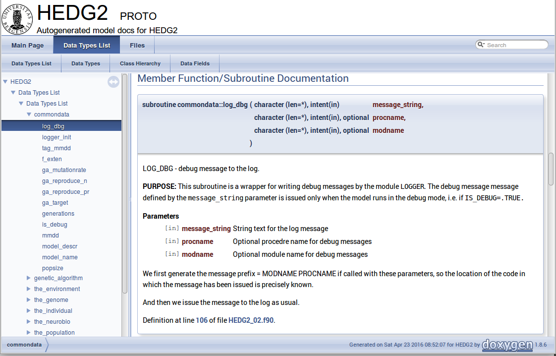
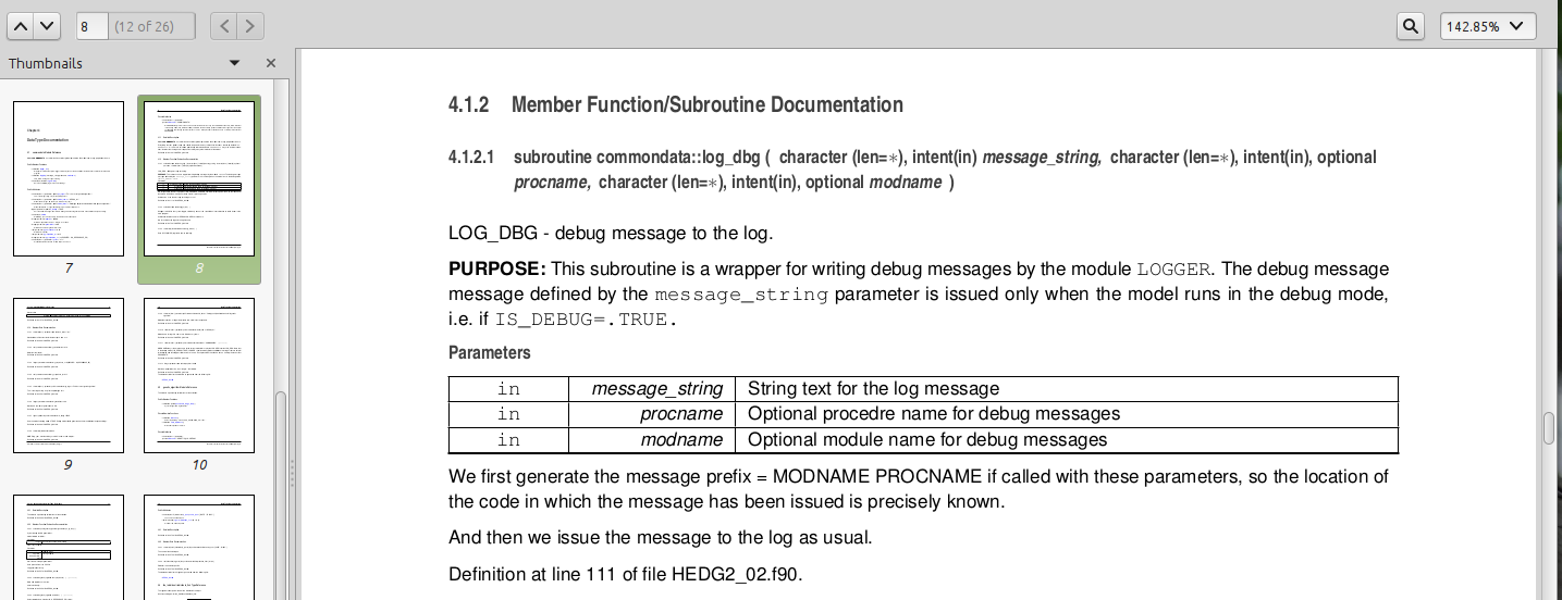
There are different options to generate HTML documents. For example, a bundle of HTML files with images , cross-references, code syntax highlighting and search functionality can be prepared. Alternatively, a single simpler HTML file can be done. LaTex output can be converted to PDF with references and index.
Examples of HTML and PDF outputs are below.
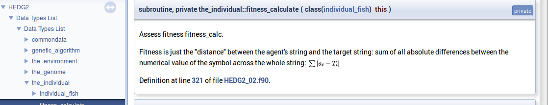
Here is an example of LaTeX formula in the autogenerated documentation file. Note that formulas are delimited with @f$ on both sides.
!> Fitness is just the "distance" between the agent's string and the target
!! string: sum of all absolute differences between the numerical value of
!! the symbol across the whole string: @f$ \sum |a_i - T_i| @f$
this%fitness = sum([(abs(iachar(this%str(i:i)) - iachar(GA_TARGET(i:i))), &
                     i = 1, len(GA_TARGET))])
This is rendered as follows:
To make the formula appear on a separate line, delimit it within @f[ and @f].
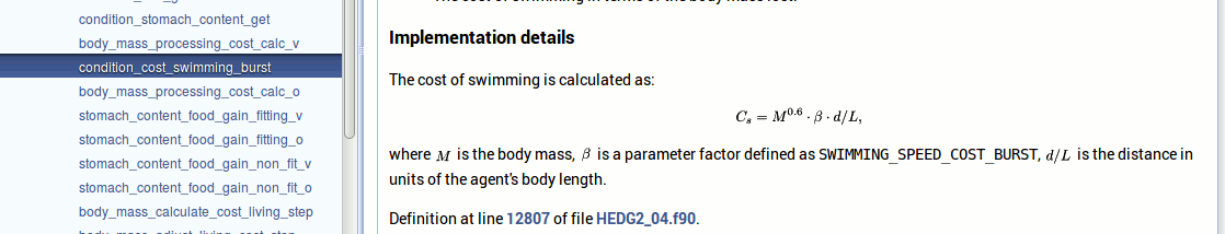
!> ### Implementation details ###
!> The cost of swimming is calculated as:
!! @f[ C_{s} = M^{0.6} \cdot \beta \cdot d / L , @f] where
!! @f$ M @f$ is the body mass, @f$ \beta @f$ is a parameter factor
!! defined as `SWIMMING_SPEED_COST_BURST`, @f$ d / L @f$ is the distance
!! in units of the agent's body length.
cost_swimming = this%body_mass**SWIM_COST_EXP * SWIMMING_SPEED_COST_BURST &
                    * distance / this%body_length
|
|
LaTeX, dvips and Ghostscript should be installed for the formula rendering to work correctly. There are web-based LaTeX equation editors, e.g. https://www.codecogs.com/latex/eqneditor.php |
Documenting a complex model is very important! It is also not really difficult, but requires some additional discipline. It is much easier to include Doxygen comments as you write the model code than to look through the whole (huge) amount of the code a month later just to recall what the code is actually doing. Thus, the model becomes much more understandable to the level of its finest details. And Doxygen allows inclusion of various markup commands and styles, LaTeX formulas and graphics. Doxygen documentation, faq’s and howtos are available here: http://doxygen.org
In the AHA GNU make system used to build the executables, documentation is generated using this simple command:
make docs
4. Version control: Subversion (SVN)
AHA Repository: https://tegsvn.uib.no/svn/tegsvn/
AHA Tools stable version (v1.1): https://tegsvn.uib.no/svn/tegsvn/tags/HEDTOOLS/1.1
4.1. Main terms
-
Working copy: the local file system directory that keeps the files synced with the Subversion server: your local copy of the code.
-
Checkout: download the files from the Subversion server initially, this sets up all the necessary data and configuration within the chosen working copy. Checkout is done only once.
-
Update: get the files with the latest changes from the Subversion server to the local file system directory (load). Files that you have changed locally and not yet committed to the server are kept intact, so your changes are never silently overwritten. To cancel all local changes use revert.
-
Commit: save the local changes to the files in your working copy to the Subversion server.
4.2. Overview
Subversion (SVN) is a version control system used in the AHA project. Use version control not only for just managing versions, but also for organising your coding. Every new code commit should ideally be a specific task, function or logical workflow unit. And the commit message should reflect this task.
For example, it would be perfect to commit changes in pieces involving implementation of a specific function in the model or to correct a specific bug. Use the log messages to describe briefly what has been done.
The usefulness of the whole version control workflow is limited if the commit pattern is haphazard and any single commit involves different kinds of code changes in many different places. It will be, for example, very difficult to revert from a single change that have previously introduced a bug. Revision history is a very valuable component of the development process!
If several people are working on the same piece of code, it is important to make commits frequently. Also frequently integrate others' changes. Otherwise, there is an increasing change to get version conflicts that have to be solved manually.
|
|
Never use the standard tools provided by the operating system (e.g. Windows Explorer) to delete/copy/move/rename files managed by Subversion. Always use the Subversion for all file operations. |
|
|
Always try to commit some logically integrated piece of code rather than do it haphazardly. Write informative commit messages. Commit changes frequently. |
The examples below assume you use a terminal console, but most SVN commands can also be easily performed from various GUI tools.
For example, imagine you add a neural response function. Commit the change, as soon as it is ready then (with log message like "Added general neural response function for neural bundles"). Go to the next logical piece of the work (e.g. fixing gamma2gene) afteer this commit and again commit this change when more or less ready (i.e. go to the next step only after you have commited the current changes). Then the versions you have will be organised into meaningful pieces:
svn commit model1.f90 -m "Added general neural response function for neural bundles"
.....
svn commit model1.f90 -m "Fixed gamma2gene function, Gaussian perception error"
A typical SVN repository organisation usually includes many branches for different purposes created by different developers. For example, the current TEG svn repo has this structure:
|-- branches                  # Private development branches
|   |-- budaev
|   |-- gabby
|   |-- henrik
|   `-- judy
|-- hormones_v2               # The hormone models and other models (below)
|   |-- branches_camilla
|   |-- branches_jacqueline
|   |-- stochastic_trunk
|   |-- stochastic_trunk_mortality
|   |-- stochastic_trunk_mortality (a & b)
|   |-- stochastic_trunk_mortality (a & b) - TEST
|   |-- tests
|   `-- trunk
|-- mesopelagic_latitude
|   |-- branches
|   |-- mesopelagic_barrier
|   |-- mesopelagic_lifehistory
|   `-- trunk
|-- nansen_seaice
|   `-- trunk
|-- pacificherring
|   |-- branches
|   `-- trunk
|-- sexevolution
|   `-- testingsexevolutionfortran
|-- tags                      # General-purpose modelling components (versions)
|   |-- AHA_R
|   |-- BINARY_IO
|   |-- CSV_IO
|   |-- HEDTOOLS
|   |-- LINEARFIT
|   |-- QSORT
|   |-- UPTAKEMM
|   `-- VISRANGE
`-- trunk                     # Accessory components (e.g. web server config)
    |-- AHAWEB
    |-- BOOKS
    |-- DOCS
    |-- scripts
    `-- SVNSERVER
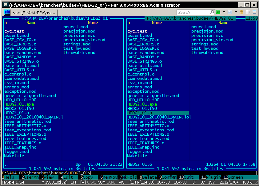
The HEDTOOLS folder itself has the following structure
`-- HEDTOOLS          # Main place for the source files
    |-- doc           # Documentation for HEDTOOLS
    |-- IEEE          # Non-intrinsic IEEE math modules
    `-- template      # Templates for user Makefile's and
                      #   HPC cluster batch scripts
Nonetheless, Subversion does not impose any limitations on the structure of directories and folders. The main advantages of Subversion over other version control systems is its simplicity and safety. One needs to know only a few commands (which can be called via graphical user interfaces) and it is virtually impossible to damage the data and code once it has gone to the server.
4.3. First time setup of the working copy
|
|
AHA Tools in (release 1.1) can be found here:
https://tegsvn.uib.no/svn/tegsvn/tags/HEDTOOLS/1.1;
Development versions are here:
https://tegsvn.uib.no/svn/tegsvn/branches/budaev/HEDTOOLS/.
So standard checkout (the stable version) is like this: svn co https://tegsvn.uib.no/svn/tegsvn/tags/HEDTOOLS/1.1 HEDTOOLS |
4.3.1. Command line tool
First time setup of the working copy of the model (working directory):
-
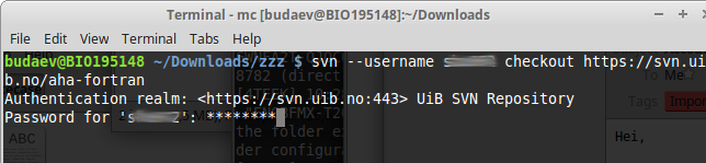
For a new project (run/experiment etc.), get into the working directory where the model code will reside (cd) (possibly make a new directory mkdir), and checkout: get the model code (one branch, no need to get everything!) from the server with svn checkout https://path_to_branch. When a specific repository is used for the first time, you should also include the user name for this repository (--username your_user_name) and then the program asks for the password. SVN server name, username and password is then saved, so subsequently it is not necessary to state the username/password you connect to the same SVN server from the same workstation. For example, first time checkout (for user u01):
svn --username u01 checkout https://tegsvn.uib.no/svn/tegsvn/branches/budaev/HED18
next, just this should work:
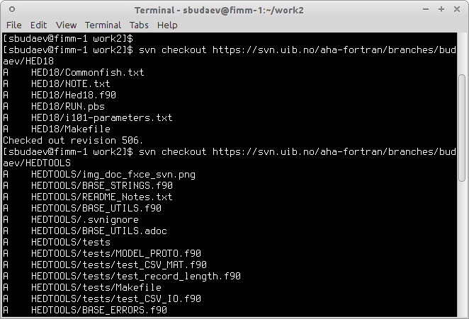
svn checkout https://tegsvn.uib.no/svn/tegsvn/branches/budaev/HED18
This will get the HED18 into the directory HED18 within the current working directory. If we use HEDTOOLS, it should also be placed here:
svn checkout https://tegsvn.uib.no/svn/tegsvn/branches/budaev/HED18
...
svn checkout https://tegsvn.uib.no/svn/tegsvn/branches/budaev/HEDTOOLS
So, we now get HED18 and HEDTOOLS in our working directory.
4.3.2. TortoiseSVN on Windows
-
Using the TortoiseSVN on Windows, initial setup is also simple.
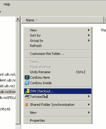
First, choose some folder for keeping the working copies of the development files, open it in the Windows Explorer.
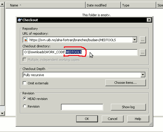
Then right-click somewhere within this folder, then choose TortoiseSVN and click Checkout. This will bring a window to enter the Subversion repository address. Now paste the address of the folder you are going to clone on the local machine. It is perhaps good to get the HEDTOOLS modelling tools initially as they are used anyway.
|
|
Unlike the command line client, TortoiseSVN by default clones to the repository directory into the current folder and does not create local folder with the same name as the remote one. |
It may therefore be necessary to retype the local directory name the same as the remote one:
Initially the system will also ask for the username and password.
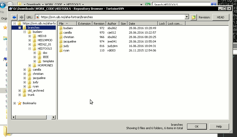
Repository browser that is called in the Checkout menu … button is a tool to explore the contents of the repository on the server. In Checkout menu it can be used to select the folder project to be cloned to the local machine. Also, using Repository browser you can make a private project directory on the server under /branches/your_name and then clone it to the local system using the Checkout menu.
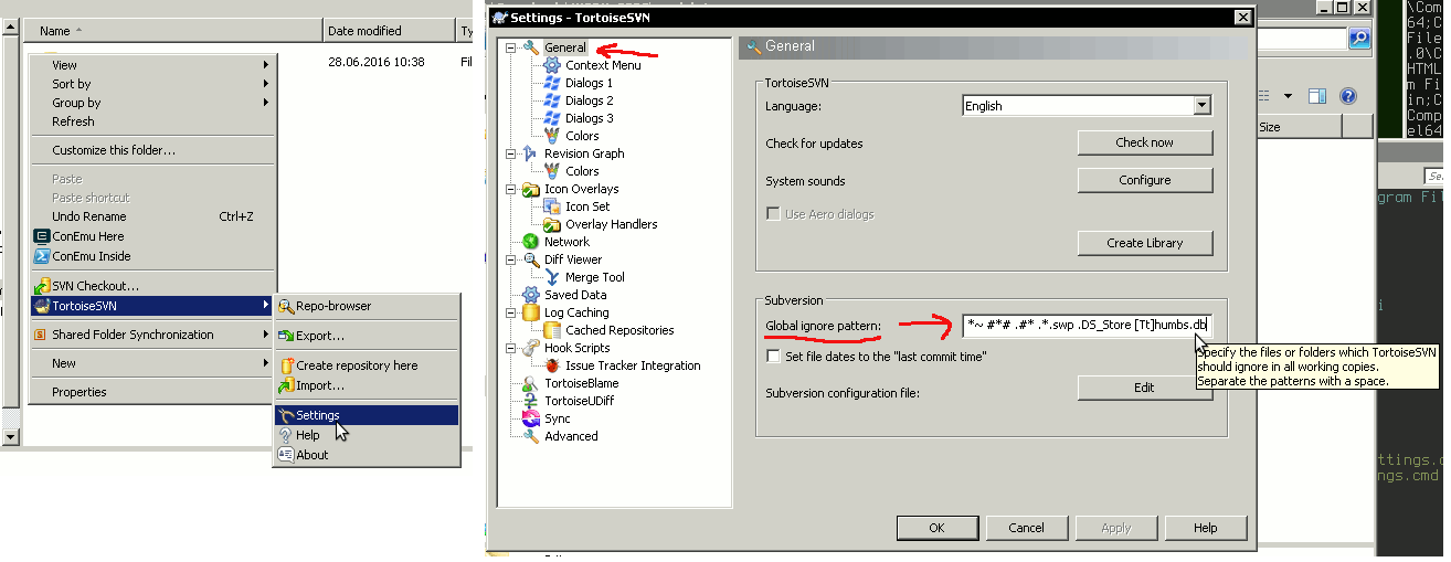
Alternatively, you can create project on the local machine first and use the menu item Import to import it to the repository. However, in the later case make sure you include only the Fortran (Matlab etc) program code into the Subversion and do not include the many accessory files created by the Microsoft Studio. They make clutter and are not needed in the versioning sytem. Use the TortoiseSVN → Settings → Ignore manu item for setting up ignore file patterns.
4.4. Standard workflow
Now you can work within this directory. This is the standard workflow.
-
update code from the server: svn up
-
edit the code using any favoured tools, build, run model etc…
-
diff (svn diff) to check what are the differences between the local file(s) or directory and those in the repository, to use specific visual diff tool use --diff-cmd diff_tool.
-
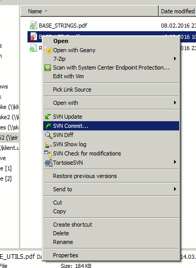
commit when ready (e.g. when a new piece of code has been implememnted): svn commit
commit will ask you to provide a short descriptive log message. It will run the standard text editor for this by default (can be configured). But you can provide such a message just on the command line with the -m option:
svn commit Hed18.f90 -m "New sigmoid function"
Both update and commit can be done for the working directory as well as for specific file. E.g. to commit only the model code Hed18.f90 do:
svn commit Hed18.f90
Both update and commit can be performed within any subdirectory of the working copy. In such cases they are limited to this subdirectory only.
4.5. Log of changes
The svn log command will issue the list of log messages, by default in the reverse order (the most recent logs go first), so the development progress is seen. The log messages can be filtered by date, revision number etc. Check out svn help log.
Example: To show only 5 most recent log messages for the specific file Hed18.f90 use such a command:
svn log -l 5 Hed18.f90
|
|
There is a small caveat with svn log. By default it shows log messages from the local working copy (not repository). So, if you did many commits lately but did not svn update, the latest messages will be absent from the log. So, do svn update! |
There is a useful utility svn2cl that generates standard GNU-style ChangeLog file. This utlity can be found in the standard Debian-based Linux repositories (subversion-tools). So, installation is trivial on Linux. Download it from the official site: svn2cl.
Example: The command below produces a slightly more concise daily log.
svn2cl --group-by-day
4.6. Using branches
A branch in Subversion is just a directory on the SVN server. It can be thought of in the same way as common file system directory/folder. Creating a new folder is easy:
# Making a new directory for old code -- use the mkdir command
svn mkdir https://tegsvn.uib.no/svn/tegsvn/old_archived
It is also easy to move or copy parts of the repository across the repository:
# Move a model branch to the archive folder -- use mv (move) command
svn mv https://tegsvn.uib.no/svn/tegsvn/trunk/model_20151013 \
      https://tegsvn.uib.no/svn/tegsvn/old_archived/model_20151013
....
# Copy a file to another branch -- use cp (copy) command
svn cp https://tegsvn.uib.no/svn/tegsvn/trunk/hormones/Hormones.f90 \
  https://tegsvn.uib.no/svn/tegsvn/branches/camilla/hormones/Hormones.f90
Do not forget to update the local working copy after deleting/moving/copying directories on the SVN server, then local copy will be in sync with the server.
4.6.1. Make a branch copying old code
The copy command is very useful to create a copy of some repository part to a separate branch. Then some new features or functions can be implemented in the branch and then reintegrated back to the parent project. Or an independent new model can be initialised in such a way.
Making a branch is easy, use svn copy source_svn_path destination_svn_path to do this. For example, the following command makes a copy of the whole sub-tree for the model code HED18 from user budaev private branch to the user natasha private branch. Now natasha can work on her own copy of the code and, when done, merge the changes back to budaev's code. Finally, budaev's (and natasha's) code can be reintegrated back to the trunk main line.
svn copy https://tegsvn.uib.no/svn/tegsvn/branches/budaev/HED18 \
    https://tegsvn.uib.no/svn/tegsvn/branches/natasha/HED18 \
    -m "Creating private branch."
4.6.2. Merge changes between branches
If several people are simultaneously working on the project, it make sense to merge changes from the parent branch back to the current branch (e.g. from trunk to budaev and natasha). Thus does not allow the code to diverge too far and reduces the chances to get version conflicts. Merging ongoing changes from the parent project is easy. For example, the following will merge changes from trunk back to the current branch (note that ^ substitutes the SVN repository web address):
svn merge ^/trunk/HEDTOOLS/
That is, with this syntax we have provided the source for merging (^/trunk/HEDTOOLS/) into the current directory.
Merge can be conducted in both ways (to and from different branches to keep them in sync). This is the main component in branch maintenance. And it is quite trivial. Make a branch — merge changes from trunk or another branch.
To undo a merge that has not yet been committed to the server, e.g. if it was done by mistake in a wrong directory, do this:
svn revert -R .
4.7. Other features
Keywords. Subversion has a very useful feature: you can set various properties (svn propset). For example, one can set tags on files or directories. A very interesting feature is that svn:keyword properties can be incorporated into the source files under SVN control. For example, you can include specific tags into the Fortran (or any other managed) source code so that they are updated automatically.
One user case for this is this. Define special $Id tag. This tag includes the file name, last changed revision number, revision date and time and the user who did the revision. This is how it will appear in the source code:
! The comment below incorporates SVN revision ID, it should apparently be
!   inserted into a comment, so does not affect the compiler:
! $Id: HEDTOOLS.adoc 19463 2025-10-17 12:08:02Z sbu062 $
!                                                          other code follows...
......
implicit none
...
To set up this tag we just have to issue such command:
svn propset svn:keywords "Id" file_name_to_set_keyword.f90
and include two strings $Id anything in between initially $ in this source text to set where the keywords should be placed. Obviously, we have to commit change to the server after this. From now on, the information will be updated automatically between the $Id … and $ symbols. So the source code itself will have comments indicating the revision number etc. There are many useful tags that can be placed in such a way. For example $Date $Revision $HeadURL $LastChangedDate. If several tags should be placed, one can set up several keywords for a particular file:
svn propset svn:keywords "Id Date Revision HeadURL LastChangedDate" file_name.f90
Check out full documentation in the SVN manual about propset and svn:keyword.
|
|
Subversion keywords are case sensitive, so $ID or $id won’t work. |
Change Subversion main repository address. If the main svn repository address is changed for some reason, svn relocate command is useful:
svn relocate --username user_name https://tegsvn.uib.no/svn/tegsvn/
TortoiseSVN client on Windows has a Relocate menu item under TortoiseSVN.
WebDAV access. It is possible to access the Subversion repository using the standard WebDAV protocol (https://) as a virtual folder without installing any client software. WebDAV is supported by most operating systems, including Windows and Linux. On Windows, use the "Map network drive"" menu to establish connection to the server. On Linux, just place such an address in the file manager ("Ctrl L" may be required to go to the address line): davs://tegsvn.uib.no/svn/tegsvn/
4.8. GUI Tools
Using the GUI tools like TortoiseSVN is similar to using the terminal commands. With GUI you should just select the appropriate item from the menu list.
Initial setup for the repository in TortoiseSVN is simple.
Checking changes, diff-ing, setting properties and keywords etc. is also very easy and visual with the built-in tool. Another useful feature is the revision graphs showing sequence of versions and pattern of branching. TortoiseSVN is incorporated into the Windows explorer and uses small overlay icons to show the status of the files and directories.
Similar GUI tools, although not as mature as TortoiseSVN, exist for Linux. For example, there is thunar-vcs-plugin (Git and Subversion integration into the Thunar file manager).

Subversion also integrates with numerous other tools, e.g. there is an SVN plugin for the Geany editor (GeanyVC), plugins for the Microsoft Visual Studio IDE etc.
For example, AnkhSVN is a nice free tool integrating Subversion into Microsoft Visual Studio.
Do not forget that version control systems are not only for just program code but any text-based files. So writing papers in LaTeX benefits from a built-in Subversion support in the TexStudio.
5. Object-oriented programming and modelling
5.1. General principles
Modern Fortran (F2003 and F2008 standards) allows coding in a truely object-oriented style. Object oriented style allows to define user’s abstractions that mimic real world objects, isolate extra complexity of the objects and create extensions of objects.
Object oriented programming is based on the following principles:
-
Abstraction: defining and abstracting common features of objects and functions.
-
Modularity and hiding irrelevant information: An object is written and treated separately from other objects. Details about internal functioning of the object are effectively hidden, what is important is the interface of the object, i.e. how it interacts with the external world. This reduces complexity.
-
Encapsulation: combining components of the object to create a new object.
-
Inheritance: components of objects (both data and functions) can be inherited across objects, e.g. properties the "genome" object inherited by a more general object "the individual."
-
Polymorphism: the provision of a single interface to objects of different types.
5.2. Simple basics
Stated simply, the object-oriented programming paradigm is based on the notion of object. Here object is an entity that integrates data and procedures that are implemented to manipulate these data. In the simplest case, data can be considered as the "properties"" or "attributes" that describe the object. Procedures that are linked with the object, on the other hand, provide other derived attributes of the object or describe what the object can "do".
Different objects can be arranged in various ways (e.g. form more complex objects like arrays). For instance a population of agents (another object) can be simply formed by arranging individual agents (other objects) into an array. Various agents can also interact with each other.
For example, a single "agent" object is an entity having such attributes as sex, spatial position, body mass, body length etc. It can also have such boolean attributes as "is alive" (true or false). For any such object, one can calculate instantaneous risk of predation and other transient derived properties. Also, the agent can interact with objects of various other kinds. For example, an agent can change its spatial position (its position attribute is changed), approach a food item and "eat" it (basically, absorb the mass attribute of the item, the item is destroyed thereafter). Agent can also do many other things, e.g. "die". The functions that are linked to the object are usually called methods.
When an instance of the object is created, it is initialised in a function (e.g. init) that is often called the constructor. Another procedure is sometimes implemented to destroy and deallocate the object, it is the destructor.
5.3. Type-bound procedures
Object-oriented code in modern Fortran is based on what is called type-bound procedures.
Briefly, a derived type is declared using the type keyword; it can contain several intrinsic and other derived types. Thus, a data structure is implemented.
type, public :: SPATIAL_POINT
  real(SRP) :: x, y, depth
  character(len=LABEL_LENGTH) :: label
  ....
end type SPATIAL_POINT
A procedure can then be declared that operates specifically on this derived type.
-
The first parameter this refers to the object that the procedure operates on.
-
The base object this is declared as class in the procedure, which allows to accept any extension of the this object as the first parameter. This is called "polymorphic objects."
Note that the other parameters (non this) can be declared as class or as type. In the former case, the procedure could accept any extensions (the procedure is then polymorphic) of the object, while in the latter, only this specific type (non-polymorphic procedure).
Components of the object are separated from its name with the percent sign %, e.g. the x coordinate is this%x.
function spatial_distance_3d (this, other) result (distance_euclidean)
  class(SPATIAL_POINT), intent(in) :: this
  real(SRP) :: distance_euclidean
  class(SPATIAL_POINT), intent(in) :: other
  distance_euclidean = dist( [this%x,  this%y,  this%depth],              &
                             [other%x, other%y, other%depth] )
end function spatial_distance_3d
The procedure is then included into the derived type declaration.
The name of the procedure that is implemented (e.g. spatial_distance_3d in the example above) is not directly called in calculations and can be declared private. Instead, a public interface name is declared in the derived type that defines how the procedure should be called, in the example below it is distance.
Note that the interface name can coincide for several different objects, however the actual procedure name (spatial_distance_3d) must be unique within the module that defines the derived type and its procedures.
type, public :: SPATIAL_POINT
  real(SRP) :: x, y, depth
  character(len=LABEL_LENGTH) :: label
  ....
  contains
  procedure, public :: distance => spatial_distance_3d
  ....
end type SPATIAL_POINT
Now, the procedure is called for the specific instance of the object (it comes to the procedure as the this first "self" parameter) using the public interface name (distance) rather than the "actual" procedure name (spatial_distance_3d).
type(SPATIAL_POINT) :: point_a, point_b
...
distance_between_points = point_a%distance( point_b ) ! use public interface
An extension object can be declared, using the extends keyword, that will use all the properties and type-bound procedures of the base object and add its own additional ones. All the data attributes (x, y, depth) of the base class SPATIAL_POINT are now defined (inherited) also for the new derived type SPATIAL_MOVING. Additionally, the new type can define new properties ans add new type-bound procedures.
This allows creating complex inheritance hierarchies across objects.
type, public, extends(SPATIAL_POINT) :: SPATIAL_MOVING
  ! The following component adds an array of history of the object
  ! movements:
  type(SPATIAL_POINT), dimension(HISTORY_SIZE_SPATIAL) :: history
  ...
  contains
    ....
    procedure, public :: go_up => spatial_moving_go_up
    procedure, public :: go_down => spatial_moving_go_down
    ....
end type SPATIAL_MOVING
It is also possible to redefine the type-bound procedures for the new derived type. For example, a subroutine init can be defined for the base type SPATIAL_POINT that sets the default x, y and depth. A different type-bound procedure with the same public interface init defined for the SPATIAL_MOVING extended type can then set the default x, y and depth and, in addition, a default move. When such init procedure is called, the result of the computation is based on the exact nature of the object on which the procedure is executed. This is called procedure overloading for a polymorphic object.
call instance_object%init()
-
If the instance_object is SPATIAL_POINT, the init procedure defined for SPATIAL_POINT is executed on the object;
-
if the instance_object is SPATIAL_MOVING, the init procedure defined for SPATIAL_MOVING is executed.
5.4. Module structure
The structure of a module that defines an inheritance hierarchy of objects and their type-bound functions is like this. The module skeleton below implements also two init procedures such that spatial_moving_init overloads the spatial_init.
module SPATIAL_OBJECTS
  ! Declarations of objects:
  type, public :: SPATIAL_POINT
    real(SRP) :: x, y, depth
    character(len=LABEL_LENGTH) :: label
    ....
    contains
    procedure, public :: init => spatial_init
    procedure, public :: distance => spatial_distance_3d
    ....
  end type SPATIAL_POINT
  ....
  type, public, extends(SPATIAL_POINT) :: SPATIAL_MOVING
    ! The following component adds an array of history of the object
    ! movements:
    type(SPATIAL_POINT), dimension(HISTORY_SIZE_SPATIAL) :: history
    ...
    contains
      ....
      procedure, public :: init => spatial_moving_init
      procedure, public :: go_up => spatial_moving_go_up
      procedure, public :: go_down => spatial_moving_go_down
      ....
  end type SPATIAL_MOVING
  .....
  ! other declarations
  .....
  contains
    ! Here go all the procedures declared in this module
    function spatial_distance_3d (this, other) result (distance_euclidean)
      class(SPATIAL_POINT), intent(in) :: this
      real(SRP) :: distance_euclidean
      class(SPATIAL_POINT), intent(in) :: other

      distance_euclidean = dist( [this%x,  this%y,  this%depth],              &
                                 [other%x, other%y, other%depth] )

    end function spatial_distance_3d

    subroutine spatial_init(this)
      class(SPATIAL_POINT), intent(inout) :: this
      ....
    end subroutine spatial_init

    subroutine spatial_moving_init(this)
      class(SPATIAL_MOVING), intent(inout) :: this
      ....
    end subroutine spatial_init

    ! Any other procedures

    ..........

end module SPATIAL_OBJECTS
An object or several related objects (derived types) together with their type-bound procedures are defined within the same Fortran module.
5.5. Class diagram
Relationships between different objects (classes) can be represented graphically in a class diagram. Here, a class (derived type) is represented by a box with a title that gives its name. The relationships are then depicted by several types of lines and arrows that connect these boxes.
The simplest and most widespread symbols in a class diagram are presented below.

-
inheritance shows which class is the base class and which is its extension;
-
aggregation indicates that several objects are "assembled" to create a more complex composite object;
-
composition is a strong form of "aggregation" that points to a "part versus whole" relationship."
5.6. Arrays of objects
Components of a derived type are referred using the percent symbol %, e.g. agent%sex refers to a component sex of the object agent. Both data components and "methods" are referred in this way, although methods use parentheses (e.g. parents%individual%probability_capture()).
Derived type data objects can be combined into arrays as normal intrinsic type variables. For example, the sex component of the i-th element of the array of derived type agent is referred as agent(i)%sex.
If arrays are defined at several levels of the object hierarchy, it can create quite a complex structure:
population%individual(i)%chromosome(j,k)%allele(l)%allele_value(m)
5.7. Implementation of objects
The above declarations just define an object. To use the object, we must instantiate it, i.e. create its specific instance and give it a value. This is analogous to having a specific data type, e.g. integer. We cannot use "just an integer," we need (1) to create a specific variable (variable is also an object though trivial!) of the type integer (e.g. integer :: Var_A) and (2) to assign a specific value to it (Var_A=1).
For example, the following creates two instance arrays of the type INDIVIDUAL_FISH. Both arrays are one-dimensional and have POPSIZE elements. So we now have two fish populations, generation_one and generation_two. Each individual value of such an array, e.g. generation_one(1) is an instance of the object of the type INDIVIDUAL_FISH that can be quite a complex data structure including many different data types, even arrays and lower-order derived types. So, instead of being arrays of simple values these object arrays are in fact arrays of complex data structures potentially consisting of many different data types and arrays:
type(INDIVIDUAL_FISH), dimension(POPSIZE) :: generation_one
type(INDIVIDUAL_FISH), dimension(POPSIZE) :: generation_two
We can now assign concrete values to each of the previously defined components of generation_one array, e.g.
generation_one(i)%sex = "male"          ! assign values to individual components
generation_one(i)%alive = .true.        ! of the object instance
generation_one(i)%food(j) = "spaghetti"
We can also use the subroutines and type-bound functions that we have defined within the object definitions to do specific manipulations on the object and its components:
subroutine population_init()
....

  do i = 1, POPSIZE
    call generation_one(i)%init()     ! Initialise the i-th fish object in the
  end do                              ! "generation_one" population array
                                      ! using the object-bound subroutine init
end subroutine population_init
5.8. A trivial example: Stopwatch object
Here is a trivial example implementing a stopwatch object — TIMER_CPU. The comments in the code are self-explanatory.
!> Here we define CPU timer container object for debugging and
!! speed/performance control. Therefore we can instantiate arbitrary timers
!! for different parts of the code (and also global). "Class," so can extend.
!! Using a specific timer (`timer_general`)
!! is like this: `call stopwatch%start()` to start the stopwatch, then the
!! function `stopwatch%elapsed()` returns the elapsed time.
!! @note The near-trivial nature of this object makes it ideal for learning
!!       how to implement objects. TODO: add to doc full implementation.
type, public :: TIMER_CPU
  !> Define start time for the stopwatch.
  !! @note We need to keep only the start time as raw values coming out
  !!       of `cpu_time` are machine-dependent
  !! @note It does not seem good to move `TIMER_CPU` to *HEDTOOLS* as they
  !!       are for portability (require only F90) and do not use OO.
  !!       `TIMER_CPU`  uses full OO extensible class implementation so
  !!       requires *F2003* minimum.
  real(SRP) :: cpu_time_start

  contains
    procedure, public :: start => timer_cpu_start       ! subroutine
    procedure, public :: elapsed => timer_cpu_elapsed   ! function

end type TIMER_CPU
....
....
  !=============================================================================
  ! The two procedures below are for the CPU timer / stopwatch object

  !-----------------------------------------------------------------------------
  !> Start the timer object, stopwatch is now ON.
  !! @note We do not need exact low-level time as it is machine-specific.
  subroutine timer_cpu_start(this)
    class(TIMER_CPU) :: this

    !> this turns on the CPU stopwatch
    call cpu_time(this%cpu_time_start)

  end subroutine timer_cpu_start

  !-----------------------------------------------------------------------------
  !> Calculate the time elapsed since the stopwatch subroutine was called
  !! for this instance of the timer container object. Can be called several
  !! times showing elapsed time since the grand start.
  function timer_cpu_elapsed (this) result (cpu_time_elapsed)
    class(TIMER_CPU) :: this
    !> @returns the time elapsed since `timer_cpu_start` call (object-bound).
    real(SRP) :: cpu_time_elapsed

    ! Local var
    real(SRP) :: cpu_time_finish

    !> We use the intrinsic `cpu_time` to get the finish time point.
    call cpu_time(cpu_time_finish)

    !> Elapsed time is then trivial to get.
    cpu_time_elapsed = cpu_time_finish - this%cpu_time_start

  end function timer_cpu_elapsed
Declarations for the instantiation of such an object look like this:
!> This is the stopwatch objects for global and for timing each generation
type(TIMER_CPU) :: stopwatch_global, stopwatch_generation
The use of the stopwatch objects is now rather simple:
! Start global stopwatch
call stopwatch_global%start()
....
....
! Print elapsed time in the log message;
!    check out the function stopwatch_global%elapsed() that actually gets
!    the elapsed time:
call LOG_DBG("Initialisation of generation one completed, took " //           &
                TOSTR(stopwatch_global%elapsed(), "(f8.4)") //                &
                "s since global procedure start.")
5.9. More information
Below are some books that should be referred for more information on object-oriented programming in modern Fortran.
-
Adams, J. C., et al., (2009). The Fortran 2003 Handbook. Springer.
-
Akin, E. (2003). Object-Oriented Programming via Fortran 90/95. Cambridge University Press.
-
Brainerd, W. S. (2015). Guide to Fortran 2008 Programming. Springer.
-
Chapman, S. J. (2007). Fortran 95/2003 for Scientists and Engineers. McGraw-Hill.
-
Clerman, N. S., & Spector, W. (2012). Modern Fortran: Style and usage. Cambridge University Press.
6. Introduction to the AHA Fortran modules
6.1. Overview of AHA modules
The modelling framework is build on these principles: (1) modularity, (2) extensibility, (3) portability.
The Modelling framework is composed of two separate components: (1) HEDTOOLS, modelling utilities and tools (implemented as portable Fortran modules, not object-oriented) that have general applicability and are used for data conversion, output, random number generation and execution logging. HEDTOOLS modules are designed such that they can be used in many different simulation projects, not only the AHA model; (2) The AHA model, an object oriented evolutionary agents simulation framework implementing standard reusable module components.

HEDTOOLS:
-
Module BASE_UTILS — utility functions.
-
Module CSV_IO — Data output in CSV (comma separated values) format.
-
Module BASE_RANDOM — Utilities for random number generation.
-
Module LOGGER — Logging facility.
-
Module BASE_STRINGS — String manipulation utilities.
-
Non-intrinsic IEEE modules — implement IEEE arithmetic checks and exceptions tracking.
The AHA Model
-
Module COMMONDATA Setting common parameters for the model.
-
Module THE_GENOME Implementation of the genome objects, gene, alleles, chromosomes.
-
Module THE_HORMONES Architecture of the hormones and their functions.
-
Module THE_NEUROBIO Implements neurobiological architectures based on sigmoid function, decision making and GOS.
-
Module THE_INDIVIDUAL Implements the individual agent in the final form and the individual-based model functions.
-
Module THE_POPULATION Implements the population(s) of agents.
-
Module THE_ENVIRONMENT Implements the environment and its variation.
-
Module THE_EVOLUTION Implements the genetic algorithm.
|
|
Solaris Studio Fortran compiler f95 v. 12.4 does not support all object-oriented features (most probably the type-bound functions and polymorphic classes) of the Fortran 2003 standard and does not compile the AHA model code issuing this error: f90: Internal Error, code=fw-interface-ctyp1-796. Though, it does compile the more portable non-object-oriented HEDTOOLS modules without issues. It is believed that the next major release of Oracle Studio will include full support of these Fortran features. Recent Intel and GNU compilers work as expected with all object-oriented code. |
6.2. Modules in Fortran
Module is just a piece of Fortran program that contains variable or constant declarations and functions and subroutines. Modules are defined in such a simple way:
module SOME_MODULE

character (len=*), private, parameter :: text_string = "its value"
integer :: some_variable
real, dimension(:)

contains                      ! subroutines and functions go after "contains"

  subroutine SOME_SUBROUTINE(parameters)
  ...
  end subroutine SOME_SUBROUTINE

end module SOME_MODULE
To use any variable/constant/subroutine/function from the module, the program must include the use MODULE_NAME statement:
use SOME_MODULE
....
Invoking the modules requires the use keyword in Fortran. use should normally be the first statements before implicit none:
program TEST

  use BASE_UTILS  ! Invoke the modules
  use CSV_IO      ! into this program

  implicit none

  character (len=255) :: REC
  integer :: i
  real, dimension(6) :: RARR = [0.1,0.2,0.3,0.4,0.5,0.6]
  character (len=4), dimension(6) :: STARR=["a1","a2","a3","a4","a5","a6"]

..........

end program TEST
Building the program with these modules using the command line is normally a two-step process:
build the modules, e.g.
gfortran -g -c ../BASE_CSV_IO.f90 ../BASE_UTILS.f90
This step should only be done if the source code of the modules change, i.e. quite rarely.
build the program (e.g. TEST.f90) with these modules
gfortran -g -o TEST.exe TEST.f90 ../BASE_UTILS.f90 ../BASE_CSV_IO.f90
or for a generic F95 compiler:
f95 -g -c ../BASE_CSV_IO.f90 ../BASE_UTILS.f90
f95 -g -o TEST.exe TEST.f90 ../BASE_UTILS.f90 ../BASE_CSV_IO.f90
A static library of the modules could also be built, so the other more changeable code can be just linked with the library.
|
|
Note
The examples above assume that the module code is located in the upper-level directory, so ../. The make system used to build the model cares about the HEDTOOLS modules automatically. |
7. Module: BASE_UTILS
This module contains a few utility functions and subroutines. So far there are two useful things here: STDOUT, STDERR, TOSTR, CLEANUP, and RANDOM_SEED_INIT.
7.1. Function: TOSTR
TOSTR converts everything to a string. Accepts any numeric or non-numeric type, including integer and real (kind 4, 8, 16), logical and strings. Also accepts arrays of these numeric types. Outputs just the string representation of the number. Aliases: STR (same as TOSTR), NUMTOSTR (accepts only numeric input parameter, not logical or string)
7.1.1. Basic examples
Integer:
STRING = TOSTR(12)
produces  "12"
Single precision real (type 4)
[Note that float point calculations,
especially single precision (real type 4) may introduce a rounding error]
print *, ">>", TOSTR(3.1415926), "<<"
produces >>3.14159250<<
Double precision real (type 8)
print *, ">>", TOSTR(3.1415926_8), "<<"
produces >>3.1415926000000001<<
TOSTR also converts logical type to the "TRUE" or "FALSE" strings and can also accept character string as input. In the latest case it just output the input.
7.1.2. Optional parameters
TOSTR can also accept standard Fortran format string as the second optional string parameter, for example:
print *, ">>", TOSTR(3.1415926,"(f4.2)"), "<<"
produces >>3.14<<
print *, ">>", TOSTR(12,"(i4)"), "<<"
produces >>  12<<
Lead zeroes. With integers, TOSTR can also generate leading zeros, which is useful for auto-generating file names or variable names. In such cases, the number of leading zeros is determined by the second optional integer parameter. This integer sets the template for the leading zeros, the maximum string. The exact value is unimportant, only the number of digits is used.
For example,
print *, ">>", TOSTR(10, 100), "<<"
produces >>010<<
print *, ">>", TOSTR(10, 999), "<<"
also produces >>010<<
print *, "File_" // TOSTR(10, 10000) // ".txt"
produces File_00010.txt
Verbatim format spaces. With scalar integer and real arguments, TOSTR can also retain leading spaces, when called with the third logical argument is_clean, this really makes sense when the format string specifier is used, then verbatim format specifier is used for the output . When is_clean is set to TRUE or unset (default), the function output string is cleaned of blanks, if it is FALSE, no cleanup is done. For example:
">>" // TOSTR( Output_Stats%total_vol_evacuated, "(f10.4)" ) // "<<"
! This code produces >>1.8169<<
">>" // TOSTR( Output_Stats%total_vol_evacuated, "(f10.4)", .FALSE. ) // "<<"
! produces >>    1.8169<< (verbatim format, leading blanks are not deleted)
7.1.3. Examples of arrays
It is possible to convert numeric arrays to their string representation:
real, dimension(6) :: RARR = [0.1,0.2,0.3,0.4,0.5,0.6]
.....
print *, ">>", TOSTR(RARR), "<<"
produces > 0.100000001 0.200000003 0.300000012 0.400000006 0.500000000 0.600000024<<
Fortran format statement is also accepted for arrays:
real, dimension(6) :: RARR = [0.1,0.2,0.3,0.4,0.5,0.6]
.....
print *, ">>", TOSTR(RARR,"(f4.2)"), "<<"
produces >> 0.10 0.20 0.30 0.40 0.50 0.60<<
It is possible to use array slices and array constructors with implicit do:
print *, ">>", TOSTR(RARR(1:4)), "<<"
print *, ">>", TOSTR( (/(RARR(i), i=1,4)/) ), "<<"
both produce >> 0.100000001 0.200000003 0.300000012 0.400000006<<
or using the newer format with square brackets:
print *, ">>", TOSTR( [(RARR(i), i=1,4), 200.1, 400.5] ), "<<"
produces >> 0.100000001 0.200000003 0.300000012 0.400000006 200.100006 400.500000<<
the same with format:
print *, ">>", TOSTR( [(RARR(i), i=1,4), 200.1, 400.5], "(f9.3)" ), "<<"
produces >> 0.100 0.200 0.300 0.400 200.100 400.500<<
The subroutine TOSTR is useful because it allows to change such confusing old-style Fortran string constructions as this
!print new gene pool. First make file name      !BSA 18/11/13
if (gen < 10) then
  write(gen1,2902) "gen-0000000",gen
else if (gen < 100) then
  write(gen1,2903) "gen-0000000",gen
else if (gen < 1000) then
  write(gen1,2904) "gen-000000",gen
else if (gen < 10000) then
  write(gen1,2905) "gen-00000",gen
else if (gen < 100000) then
  write(gen1,2906) "gen-0000",gen
else if (gen < 1000000) then
  write(gen1,2907) "gen-000",gen
else if (gen < 10000000) then
  write(gen1,2913) "gen-00",gen
else if (gen < 100000000) then
  write(gen1,2914) "gen-0",gen
else
  write(gen1,2915) "gen-",gen
end if

if (age < 10) then
  write(gen2,2920) "age-0000",age
else if (age < 100) then
  write(gen2,2921) "age-000",age
else if (age < 1000) then
  write(gen2,2922) "age-00",age
else if (age < 10000) then
  write(gen2,2923) "age-0",age
else
  write(gen2,2924) "age-",age
end if

write(gen3,2908)gen1,"-",gen2

if (expmt < 10) then
  write(string104,2901)"HED24-",MMDD,runtag,"-E0",expmt,"-o104-genepool-",gen3,".txt"
else
  write(string104,2910)"HED24-",MMDD,runtag,"-E",expmt,"-o104-genepool-",gen3,".txt"
end if
to a much shorter and clear like this:
!print new gene pool. First make file name      !BSA 18/11/13
string104 = "HED24-" // trim(MMDD) // trim(runtag) // "-E0" // &
            TOSTR(expmt,10) // "-o104-genepool-" // &
            "gen-" // TOSTR(gen, 10000000) //  "-" // &
            "age-" // TOSTR(age, 10000) // f_exten
7.2. Subroutines: STDOUT and STDERR
These subroutines output arbitrary text to the terminal, either to the standard output and standard error. While it seems trivial (standard Fortran print *, or write() can be used), it is still good to have a dedicated standard subroutine for all outputs as we can then easily modify the code to use Matlab/R API to work with and run models from within these environments, or use a GUI window (the least necessary feature now, but may be useful if the environment is used for teaching in future). In such cases we will then implement a specific dedicated output function and just globally swap STDOUT with something like R_MESSAGE_PRINT or X_TXTGUI_PRINT.
STDOUT/STDERR accept an arbitrary number of string parameters, which just represent messages placed to the output. Each parameter is printed on a new line. Trivial indeed:)
|
|
It is useful to have two separate subroutines for stdout and stderr
as they could be easily separated (e.g. redirected to different files).
Redirection could be done under Windows/Linux terminal in such a simple way: model_command.exe 1>output_file_stdout 2>output_file_stderr Here STDOUT is redirected to output_file_stdout, STDERR, to output_file_stderr. |
Examples
call STDOUT("---------------------------------------------------",&
            ch01 // " = " // ch02 // TOSTR(inumber) // " ***", &
            ch10 // "; TEST NR= " // TOSTR(120.345), &
            "Pi equals to = " //  TOSTR(realPi, "(f4.2)"), &
            "---------------------------------------------------")
The above code just prints a message. Note that TOSTR function is used to append numerical values to the text output (unlike standard write where values are separated by commas).
7.3. Function: CLEANUP
CLEANUP Removes all spaces, tabs, and any control characters from the input string. It is useful to make sure there are no trailing spaces in fixed Fortran strings and no spaces in file names.
Example:
print *, ">>", CLEANUP("This is along string blablabla"), "<<"
produces >>Thisisalongstringblablabla<<
7.4. Determining the runtime platform: PLATFORM_IS_WINDOWS
This function determines if the program is currently running on Microsoft Windows. If this is the case, returns TRUE, otherwise FALSE.
The detection algorithm is very simple, it just checks if the Windows standard environment variable ComSpec is set. ComSpec appears to be case sensitive on recent versions of Microsoft Windows, but this is not guaranteed.
if ( PLATFORM_IS_WINDOWS() ) print *, "Running on Windows."
7.5. Linearly spaced array: LINSPACE
This function calculates an array of values that are equally spaced in the linear space. It accepts three parameters: real minimum value, real maximum value and an integer number indicating how many values should be generated. The output array is allocatable to the size of the number of values.
print *, LINSPACE(1.0, 10.0, 10) ! 1.0 2.0 3.0 4.0 5.0 6.0 7.0 8.0 9.0 10.0
7.6. Interpolation: LINTERPOL, DDPINTERPOL, INTERP_LINEAR, INTERP_LAGRANGE, CSPLINE
LINTERPOL is a simple linear interpolation function. It takes a sorted independent variable (X) vector, a conforming (same dimensionality) dependent variable (Y) vector that set the grid data as well as a single X argument to get the dependent variable Y result of the function. An optional integer error code (with the intent out) can be provided to check errors.
Possible error code values are 0 no error; 100 input arrays not conforming; -1 the X argument is below the low limit of the grid array; 1 the X argument is above the upper grid limit; -101 input arrays not conforming and X is below low limit; 101 input arrays are not conforming and X argument is above the upper grid limit.
The grid vectors and the X argument can be real kind 4 or kind 8 values, all with same type (i.e. no kind mixing within a single function call).
print *, LINTERPOL( [1.,2.,3.,6.,12.], [0.1, 0.5, 0.7, 0.95, 0.99], 0.2, IERR )
The DDPINTERPOL function works similarly to LINTERPOL, but uses the nonlinear Divided Difference Polynomials Interpolation algorithm.
INTERP_LINEAR is a subroutine that performs linear piecewise interpolation of a whole array. It takes the following arguments: (1) independent (X) grid data vector, (2) dependent (Y) grid data vector, (3) independent data vector for interpolation, (4) the dependent vector of the resulting dependent data values.
call INTERP_LINEAR ( XDAT, YDAT, [0.002, 0.1, 0.5, 0.9, 0.95, 0.98], OUT_Y )
The INTERP_LAGRANGE subroutine works similarly to INTERP_LINEAR but performs Lagrange polynomial interpolation.
Thare are also two interpolation functions that return a vector: LIN_INTERPOL_VECTOR and LAGR_INTERPOL_VECTOR. They do, respectively, linear and Lagrange polynomial interpolation.
print *, LIN_INTERPOL_VECTOR( [1.,2.,3.,4.,5.],                               &
                              [0.1, 0.5, 0.9, 0.95, 0.98 ],                   &
                              [1.25, 1.1, 4.1, 1.9, 1.95, 1.98]  )


print *, LAGR_INTERPOL_VECTOR( [1.,2.,3.,4.,5.],                              &
                               [0.1, 0.5, 0.9, 0.95, 0.98 ],                  &
                               [1.25, 1.1, 4.1, 1.9, 1.95, 1.98]  )
The CSPLINE subroutine works similarly to INTERP_LINEAR and INTERP_LAGRANGE but performs cubic spline interpolation under the "not a knot" condition. Results from this procedure appear to be the same as in the matlab spline function. The procedure is based on original code in Slatec from Guide to Available Mathematical Software (GAMS) web site at the National Institute of Standards and Technology.
call CSPLINE ( XDAT, YDAT, XINTERPOL, vector_output )
There is also a function that returns a vector: CSPLINE_VECTOR.
ploty = CSPLINE_VECTOR( xx, yy, plotx )
7.7. Subroutines: ARRAY_INDEX and ARRAY_RANK
ARRAY_INDEX calculates an integer sorting index vector for sorting a
real (kind 4 or 8) or an integer input vector
[This routine
is based on the high performance algorithm from Michel Olagnon’s
ORDERPACK. It is also analogous to
the indexx subroutine from the Numerical recipes (very restrictive
license disallowing source code distribution).]
. The first parameter of the
subroutine defines the vector to be sorted, the second is the calculated
integer indexing vector. The input vector can then be easily sorted by the
integer sorting indices.
The routines can add the third scalar integer parameter, the maximum order to index the array. In such cases, this will result in partial indexing ordering, which is much faster if we are not interested in the whole array (e.g. intetested in finding, indexing and ranking the smallest N elements). See the code example below.
Example:
! Calculate index array for vector X
call ARRAY_INDEX(X, index_array)

! To get the vector X sorted, just use this index array by vector indexing:
print *, X(index_array)
ARRAY_RANK calculates the ranking order scores for the original vector using the integer sorting index vector that is calculated by ARRAY_INDEX.
Example:
! Calculate ranks for the input array X from the previous example.
call ARRAY_RANK(index_array, ranks_for_X)
This shows how to use ARRAY_INDEX and ARRAY_RANK together.
program TESTRANKS
  use BASE_UTILS
  integer :: i               ! Original vector X to sort and rank:
  real(4), dimension(10) :: X=[ 13.,12.,14.,11.,15.,99.,16.,18.,17.,19.]
  integer, dimension(10) :: Id = 0, Ranks

  call ARRAY_INDEX(X, Id)    ! Calculate index vector for X:
                             !   4   2   1   3   5   7   9   8  10   6
  call ARRAY_RANK(Id, Ranks) ! Calculate rank scores for the original vector X:
                             !   3   2   4   1   5  10   6   8   7   9
end program TESTRANKS
The code below shows partial indexing:
program TESTRANKS
  use BASE_UTILS
  integer :: i
  real(4), dimension(10) :: X=[ 13.,12.,14.,11.,15.,99.,16.,18.,17.,19.]

  integer, dimension(10) :: Id = 0, Ranks

  integer :: order

  order=7                          ! Set the order, indexing is done up to this.
  if (order>size(X)) order=size(X) ! Order must be smaller than the vector, the
                                   ! indexing procedure does NOT auto-check it.

  Id=-9999; Ranks=-9999            ! Note that we need to initialise the index
                                   ! vector before use to avoid errors, depends
                                   ! on how compiler treats uninitialised arrays.

  call ARRAY_INDEX(X, Id, order)   ! Calculate index vector for X:
                                   !  4  2  1  3  5  7  9  -9999 -9999 -9999
  call ARRAY_RANK(Id, Ranks)       ! Calculate rank scores for the original X:
                                   !  3  2  4  1  5  -9999  6  -9999 7  -9999
  print *, Id
  print *, Ranks

end program TESTRANKS
7.8. Subroutines: ARRAY_QSORT
ARRAY_QSORT sorts a one-dimensional array (vector), in an increasing (default) or decreasing order. The array can be integer or real type.
integer [real], intent(inout), dimension(:) :: A ! Input array to be sorted
logical, optional, intent(in) :: is_reverse      ! Optional flag requesting
                                                 !   decreasing sort
Example
integer, dimension(10) :: intarray = [1,4,6,1,0,0,8,3,4,5]
...
call ARRAY_QSORT(intarray)          ! [0,0,1,1,3,4,4,5,6,8]
...
call ARRAY_QSORT(intarray, .TRUE.)  ! [8,6,5,4,4,3,1,1,0,0]
7.9. Function: ZEROFUN
ZEROFUN calculates a zero of an arbitrary function F(X) (that is passed as an argument) in specific interval (from AX to BX).
real, intent(in) :: AX    ! Lower limit of the search interval
real, intent(in) :: BX    ! Upper limit of the search interval
real             :: F     ! A function that is searched. This must be
                          ! implemented as a Fortran function
real, intent(in) :: TOL   ! Numerical tolerance
The real arguments can be "single" (kind 4) or "double" (kind 8) precision.
The function that is passed as an argument should be a module procedure or external declared in an interface block.
For more details see:
-
Brent, R.P., (1973). Algorithms for mnimization without derivatives, Prentice-Hall, Inc.
-
Brent, R.P. (1971). An algorithm with guaranteed convergence for finding a zero of a function, Computer J. 14, 422–425.
Example
! Find zero value of f(x) = X**3 - 2 at the interval (-2,2)
A = -2.0_SP;
B =  2.0_SP;
Y = ZEROFUN(A, B, cubic, eps_f)

...

function cubic(x) result (y)
  use m_tests
  real(SP), intent(in) :: x
  real(SP) :: y
  y = x ** 3 - 2.0
end function zf_qubic_r4
Example
! Call of ZEROFUN
depth_out = ZEROFUN( depth_range_min_loc,                                  &
                     depth_range_max_loc,                                  &
                     visibility_loc_diff,                                  &
                     TOLERANCE_HIGH_DEF_SRP )
...

  ! This function is passed as an argument into ZEROFUN
  real(SRP) function visibility_loc_diff(depth)
    !> @param[in] depth the depth of the spatial object.
    real(SRP), intent(in) :: depth
    visibility_loc_diff = visibility_loc(depth) - target_range
  end function visibility_loc_diff
7.10. Subroutine: RANDOM_SEED_INIT_SIMPLE
RANDOM_SEED_INIT_SIMPLE is called without parameters and just initialises the random seed for the Fortran random number generator. But note that the module BASE_RANDOM contains a much better subroutine RANDOM_SEED_INIT that is also suitable for parallel processing systems (RANDOM_SEED_INIT_SIMPLE cannot be used in parallel calculations).
Example
call RANDOM_SEED_INIT
8. Module: CSV_IO
8.1. Overview
This module contains subroutines and functions for outputting numerical data to the CSV (Comma Separated Values) format (RFC4180, CSV format). There are many procedures for data output to CSV, and only CSV_MATRIX_READ for input (we don’t input much data).
CSV is especially useful because it is human-readable but can still be easily imported into spreadsheets and stats packages (e.g. R reads CSV natively). It also has relatively small file size overhead compared to formatted text or XML, which is good if huge amounts of data are generated by the model.
CSV record is a whole line (row) of numbers/strings (as in Excel), a single file can have quite many records (rows).

For example, records (rows) can represent consecutive generations during the evolution or individuals for within-generation data.
In a typical workflow, within-column variables (i.e those that belong to the same row of data file) are appended to the same record. When the record is full (i.e. the number of values appended is equal to the number of columns in the CSV file), the record is written physically to the disk file and we can go to writing the next record (row) of the data.
Such a workflow can be like this:

Thus, subs ending with _WRITE and _CLOSE do physical write.
This module is most suited at this moment for CSV file output rather than input.
This module widely uses optional arguments. They may or may not be present in the function/subroutine call. If not all parameters are passed, so called named parameters are used. That is, the name of the parameter(s) within the function is explicitly stated when the function/subroutine is called.
For example, GET_FREE_FUNIT has its both parameters optional (max_funit and file_status), it can be called in the standard way as below:
intNextunit = GET_FREE_FUNIT(200, logicalFlag)
It can lack any parameter:
intNextunit = GET_FREE_FUNIT()
If the first optional parameter is absent, GET_FREE_FUNIT is called as here:
intNextunit = GET_FREE_FUNIT(file_status=logicalFlag)
If both parameters present but swapped in order, it should be
intNextunit = GET_FREE_FUNIT(file_status=logicalFlag, max_funit=200)
of course, it can also be used this way:
intNextunit = GET_FREE_FUNIT(max_funit=200, file_status=logicalFlag)
|
|
The standard way of using subroutine parameters (without explicitly setting their names) when calling subroutine works only when their are not missing and their order remains the same as in the subroutine declaration. When a function / subroutine has many parameters and optional are interspersed with mandatory, it is probably just safer to use named parameters anyway. |
Files can be referred either by unit or by name, but unit has precedence (if both a provided, unit is used). There is also a derived type csv_file that can be used as a single file handle. If csv_file object is defined, the file name, unit and the latest operation success status can be accessed as %name, %unit, %status (e.g. some_file%name, some_file%unit).
The physical file operation error flag, csv_file_status is of logical type. It is always an optional parameter.
Here is an example of the data saving workflow:
use CSV_IO  ! invoke this module first
........
........
! 1. Generate file name for CSV output
csv_file_append_data_name="data_genomeNR_" // TOSTR(i) // "_" // TOSTR(j) // &
                          "_" // TOSTR(k) // ".csv"
........
! 2. open CSV file for writing
call CSV_OPEN_WRITE (csv_file_append_data_name, csv_file_append_data_unit, &
                     csv_written_ok)
if (.not. csv_written_ok) goto 1000 ! handle possible CSV error
! 3. Write optional descriptive header for the file
call CSV_HEADER_WRITE(csv_file_name = csv_file_append_data_name, &
                      header = header_is_from_this_string, &
                      csv_file_status = csv_written_ok)
........
........
! 4. Generate a whole record of variable (column) names
record_csv="" ! but first, prepare empty record string
call CSV_RECORD_APPEND(record_csv,["VAR_001", ("VAR_" // TOSTR(i,100),i=2,Cdip)])
! 5. physically write this variable header record to the file
call CSV_RECORD_WRITE (record=record_csv, &
                       csv_file_name=csv_file_append_data_name,&
                       csv_file_status=csv_written_ok)
if (.not. csv_written_ok) goto 1000 ! handle possible CSV error
........
........
! 6. Now we can write records containing actual data values, we do this
!    in two do-loops
CYCLE_OVER_RECORDS: do l=1, Cdip
  ! 7. Prepare an empty string for the current CSV record
  record_csv=""
  CYCLE_WITHIN_RECORD: do m=1, CNRcomp
    ....
    ! do some calculations...
    .....
    .....
    ! 8. append the next value (single number: genomeNR) to the current record
    call CSV_RECORD_APPEND ( record_csv, genomeNR(l,m) )
    .....
  end do CYCLE_WITHIN_RECORD
  ! 9. physically write the current record
  call CSV_RECORD_WRITE ( record=record_csv, &
                          csv_file_name=csv_file_append_data_name,&
                          csv_file_status=csv_written_ok )
  if (.not. csv_written_ok) goto 1000 ! handle possible CSV error
  .......
end do CYCLE_OVER_RECORDS
! 10. close the CSV file when done
call CSV_CLOSE( csv_file_name=csv_file_append_data_name, &
                csv_file_status=csv_written_ok )
if (.not. csv_written_ok) goto 1000 ! handle possible CSV error
The code below illustrates how the whole process
use CSV_IO
use BASE_UTILS, only : TOSTR

integer :: i, j, num

! This c_file defines file handle for CSV
type(csv_file) :: c_file

! WARNING: the record string variable cannot be allocatable
character(255) :: c_record

num = 0

! File handle must at least define the file name
c_file%name = "test_2.csv"

call CSV_OPEN_WRITE(c_file)

! Create and write the varable names
c_record=""
do i = 1, 5
  call CSV_RECORD_APPEND(c_record, "VAR_" // TOSTR(i))
end do
call CSV_RECORD_WRITE(c_record, c_file)

! Write rows
do i =1, 10
  c_record = ""
  ! Write columns within each row
  do j = 1, 5
    ! we output values of num
    num = num + 1
    call CSV_RECORD_APPEND(c_record, num)
  end do
  call CSV_RECORD_WRITE(c_record, c_file)
end do

call CSV_CLOSE(c_file)
This results in the following data file output:
"VAR_1","VAR_2","VAR_3","VAR_4","VAR_5"
1,2,3,4,5
6,7,8,9,10
11,12,13,14,15
16,17,18,19,20
21,22,23,24,25
26,27,28,29,30
31,32,33,34,35
36,37,38,39,40
41,42,43,44,45
46,47,48,49,50
Additionally, there is a wrapper for saving the whole chunk of the data at once. A whole array or matrix (2-dimensional table) can be exported to CSV in a single command:
! save the whole matrix/array d_matrix to some_file.csv
call CSV_MATRIX_WRITE(d_matrix, "some_file.csv", fstat_csv)
if (.not. fstat_csv) goto 1000
An extended example code sthat illustrates how to write diverse data to a single CSV file is found in the Extended example section.
8.2. Subroutine: CSV_OPEN_WRITE
Open CSV file for writing. May have two forms:
(1) either get three parameters:
character (len=*) :: csv_file_name  ! file name
integer :: csv_file_unit            ! file unit
logical :: csv_file_status          ! optional status flag, TRUE if operation
                                    !   successful
(2) get the (single) file handle object of the derived type csv_file
type(csv_file), intent(inout) :: csv_file_handle ! file handle object
Example
type(csv_file) :: file_occ      ! declare file handle object
........
call CSV_OPEN_WRITE(file_occ)   ! use file handle object
........
call CSV_OPEN_WRITE(file_name_data1, file_unit_data1, fstat_csv) ! old style
 if (.not. fstat_csv) goto 1000
8.3. Subroutine: CSV_CLOSE
Closes a CSV file for reading or writing. May have two forms:
(1) either get three optional parameters:
character (len=*) :: csv_file_name  ! file name
integer :: csv_file_unit            ! file unit
logical :: csv_file_status          ! optional status flag, TRUE if operation
                                    !   successful
|
|
At least file name or unit should be present in the subroutine call. |
(2) get one file handle object of the derived type csv_file
type(csv_file), intent(inout) :: csv_file_handle ! file handle object
Example
type(csv_file) :: file_occ          ! declare file handle object
........
call CSV_CLOSE(file_occ)            ! use file handle object
........
call CSV_CLOSE(csv_file_name=file_name_data1, &   ! old style
               csv_file_status=fstat_csv)
 if (.not. fstat_csv) goto 1000
8.4. Subroutine: CSV_HEADER_WRITE
Writes an optional descriptive header to a CSV file. The header should normally be the first line of the file.
May have two forms:
(1) either get four parameters, only the header is mandatory, but the file must be identified by name or unit:
character (len=*) :: csv_file_name  ! file name
integer :: csv_file_unit            ! file unit
character (len=*) :: header         ! header string
logical :: csv_file_status          ! status flag, TRUE if operation successful
|
|
At least file name or unit should be present in the subroutine call. |
(2) get two parameters including the header string and the file handle object of the type csv_file
character (len=*) :: header         ! mandatory CSV file header
type(csv_file) :: csv_file_handle   ! file handle object
Example
call CSV_HEADER_WRITE(csv_file_name=FILE_NAME_CSV1, &
      header="Example header. Total " // TOSTR(CSV_RECORD_SIZE(record_csv)) // &
      " columns of data.", csv_file_status=fstat_csv)
if (.not. fstat_csv) goto 1000
Here CSV file header is generated from several components, including the CSV_RECORD_SIZE function to count the record size.
8.5. Function: GET_FILE_UNIT
Returns file unit associated with an existing open file name, if no file unit is associated with this name (file is not opened), return unit=-1 and error status
Input parameters:
character (len=*) :: csv_file_name    ! mandatory file name
logical :: csv_file_status            ! optional status flag, TRUE if operation
                                      !   successful
Output parameter (function value):
integer :: csv_file_unit ! unit associated with open file name
Example
file_unit = GET_FILE_UNIT(file_name)
8.6. Function: GET_FREE_FUNIT
Returns the next free/available Fortran file unit number. Can optionally search until a specific maximum unit number.
Input parameters, optional:
logical :: file_status                ! operation success status
integer :: max_funit                  ! maximum unit to search
Output parameter (function value):
integer :: file_unit ! the first free/available file unit
|
|
When optional input parameters are absent, the function uses a hardwired maximum unit number, possibly depending on the computer platform and compiler used. |
Example
restart_file_unit_27 = GET_FREE_FUNIT()
8.7. Function: CHECK_UNIT_VALID
Checks if file unit is valid, that is within the allowed range and doesn’t include standard input/output/stderr units. The unit should not necessarily be linked to any file or be an open file.
Input parameter:
integer :: file_unit ! Fortran file unit to check
Output parameter (function value):
logical :: file_status ! gets TRUE if the unit is valid
Example
if (.not. CHECK_UNIT_VALID(csv_file_unit)) then
      csv_file_unit=GET_FREE_FUNIT(csv_file_status, MAX_UNIT)
.........
In this example, we check if the user provided unit is valid, if not, get the first available one.
8.8. Function: CHECK_FILE_OPEN
Checks if a file is currently open, can optionally determine the Fortran unit associated with an open file (returns -1 if it is not open). Input parameters can be either raw form (file name or unit) or csv_file object. Optional csv_file_status can determine if the check proceeded without error (=TRUE) there was an error when trying to access the file (=FALSE). Input parameters must be either file name or unit.
Standard (verbose) form:
! Calling parameters
character (len=*), optional, intent(in) :: csv_file_name  ! file name to check
integer, optional, intent(in) :: csv_file_unit            !  or unit to check
logical, optional, intent(out) :: csv_file_status         ! error status
integer, optional, intent(out) :: get_csv_file_unit       ! obtain file unit of
                                                          !  an open file
File object form:
type(csv_file) :: csv_file_handle
Output of the function is logical type, returns TRUE if the file is currently opened, FALSE otherwise.
Examples:
if (.not. CHECK_FILE_OPEN("file_out.csv")) call OPEN_OUTPUT
...
if (CHECK_FILE_OPEN(csv_file_unit=12)) goto 100
...
file_is_open = CHECK_FILE_OPEN(csv_file_name="data_out.csv", &
                               get_csv_file_unit=fileunit,   &
                               csv_file_status=error_flag)
type (csv_file) :: output_handle
...
if (CHECK_FILE_OPEN(output_handle)) then
...
8.9. Subroutine: CSV_RECORD_APPEND
Appends one of the possible data objects to the current CSV record. Data objects could be either a single value (integer, real with single or double precision, character string) or a one-dimensional array of the above types or still an arbitrary length list of the same data types from the above list.
8.9.1. Overview
The first parameter of the subroutine is always character string record:
character (len=*) :: record ! character string record to append data
The other parameters may be of any of thee following types: integer (kind=4), real(kind=4), real(kind=8), character string.
|
|
The record keeping variable can be either fixed length string or an allocatable string. But it should fit the whole record. This might be a little bit tricky if record is allocatable as record_string="" allocates it to an empty string. A good tip is to use the repeat function in Fortran to allocate the record string to the necessary value, e.g. record=repeat(" ", MAX_RECORD) will produce a string consisting of MAX_RECORD blank characters. record should not necessarily be an empty string initially, it could be just a whole blank string. |
8.9.2. Examples
Append a single string to the current record:
call CSV_RECORD_APPEND(record_csv, "ROW_NAMES")
Note that the string value is by default quoted in the output CSV file. To avoid quoting, use optional logical parameter is_quoted set to FALSE. For example
! Here a numeric variable ratio is first converted to a formatted string and
! then appended to a CSV record without quoting. This can be a method to save
! a numeric value forcing with a specific format.
call CSV_RECORD_APPEND(record_csv, TOSTR(ratio,FFMT),is_quoted=.FALSE.)
Append a single value (any of the supported types) to the current record:
call CSV_RECORD_APPEND(record_csv, value)     ! some variable of supported type
call CSV_RECORD_APPEND(record_csv, 123.5_8)   ! double precision literal value
Append a list of values (any one of the supported types) to the current record:
call CSV_RECORD_APPEND(record_csv, fish, age, stat4, fecund)
Append an array slice (any of the supported types) to the current record:
call CSV_RECORD_APPEND(record_csv, RARR(1:4))
Append an array using old-style array constructor with implied do (any of the supported types) to the current record:
call CSV_RECORD_APPEND(record_csv,(/(RARR(i), i=1,6)/))
Append an array using new-style array constructor (square brackets) with implied do plus two other values (all values can have any of the supported types but should have the same type) to the current record:
call CSV_RECORD_APPEND(record_csv, [(RARR(i), i=1,4), measur1, age(fish)])
Append integers from 1 to 10 to the current record (using implied do):
call CSV_RECORD_APPEND(record_csv, [(i,i=1,10)])
Append a string, an array of strings with implied do and finally another string to the record. This example shows how variable (column) names could be generated:
call CSV_RECORD_APPEND(record_csv,["ROW_NAME",("VAR_" // TOSTR(i,1000),i=1,1000),"STATUS"])
|
|
On some compilers (e.g. Oracle Solaris Studio f95 v.12 but not GNU gfortran version >5), all strings within the array constructor must explicitly have the same length, otherwise the compiler issues an error. In gfortran (v>5, the first occurrence of the string (e.g. the first iteration of the implied do loop) defines the default length and all extra characters are just silently dropped. The behaviour of other compilers and their versions may differ. |
8.10. Function: CSV_GUESS_RECORD_LENGTH
Guesses the maximum size for the string variable keeping the record being appended for CSV_RECORD_APPEND.
It gets two parameters: integer record size (the number of separate numerical values in the record) and the maximum target value (integer, real, or double precision real (kind=8)) and returns an integer value for a guess for the record size. The target value is used to estimate the number of characters and should have the same type as the values being appended with CSV_RECORD_APPEND.
! suppose we have a real matrix and like to save it to a CSV file
real, dimension(1000,20) :: MATRX_A
...
! we declare the CSV record as allocatable string
character(len=:), allocatable  :: record_for_csv
...

! As explained in the Important note to CSV_RECORD_APPEND above, we have to
!   allocate the string record such that it fits the complete record;
! This can be achieved as follows. Here 20 is the record size (number of cols,
!   can be determined as ubound(MATRX_A,2)), and the target value is the
!   maximum numeric value of the matrix MATRX_A:
record_for_csv = repeat(" ", CSV_GUESS_RECORD_LENGTH(20, maxval(MATRX_A)))
|
|
Use this function with caution, especially if long strings are also added to the CSV file. In such a case, make additional allowance for the added string(s). |
8.11. Function: CSV_RECORD_SIZE
Counts the number of values in a CSV record.
Input parameters:
character (len=*) :: record ! mandatory CSV record
Function value: an integer
integer :: csv_record_size
Example
print *, "This record is: ", CSV_RECORD_SIZE(record_csv), " columns."
8.12. Function: CSV_FILE_LINES_COUNT
Counts the number of lines in an existing CSV file. If file cannot be opened or file error occurred, then issues the value -1
Input parameters:
character (len=*) :: csv_file_name  ! The name of the existing file.
logical :: numeric_only             ! Optional flag to include only numeric rows.
logical :: csv_file_status          ! Optional file operation status, TRUE if
                                    !   file operations were successful.
Function value: an integer
integer :: csv_file_lines_count ! number of lines in file, -1 if file error
Can actually calculate the number of lines in any text file. Does not distinguish header or variable names lines in the CSV file and does not recognize CSV format.
Example
print *, "File ", CSV_FILE_LINES_COUNT("test_file.csv", .TRUE., succ_flag), "lines."
8.13. Subroutine: CSV_RECORD_WRITE
Physically writes a complete record of data to a CSV file. A record is a single row of data in the file.
This subroutine has two forms:
(1) it can either accept three parameters:
character (len=*) :: csv_file_name        ! file name
integer :: csv_file_unit                  ! file unit
character (len=*)  :: record              ! current CSV record (mandatory)
logical :: csv_file_status                ! optional operation status, TRUE if
                                          !  success
|
|
The file to write the current record can be referred either by name or unit. So one of them must be present in the subroutine call. |
(2) get the CSV record and the (single) file handle object of the derived type csv_file
character (len=*)  :: record              ! current CSV record (mandatory)
type(csv_file) :: csv_file_handle         ! file handle object
Example
call CSV_RECORD_WRITE(csv_record, file_cop)               ! write current record
call LOG_MSG("Physically wrote record " // TOSTR(a) // &  ! report this in some
             " to the file " // file_cop%name // &        ! logging subroutine.
             ", write status =" // TOSTR(file_cop%status))
Note, that file handle object is used in the above example.
8.14. Subroutine: CSV_MATRIX_WRITE
Writes a matrix of real (kind 4 or 8), integer or string values to a CSV data file. This is a shortcut allowing to write data in a single code instruction. This subroutine works either with a two-dimensional matrix or one-dimensional array (vector). The behaviour is a little different in these cases.
|
|
CSV matrix subroutines use the "standard" arrangement for the matrix: the first index is for rows, the second, for columns. A reverse can be produced using the intrinsic transpose function. |
8.14.1. Two-dimensional matrix
It gets the following parameters: (1) two-dimensional data matrix (of any supported type), (2) mandatory name of the output file; (3) optional vector of column names. If the column name vector is shorter than the "column" dimension of the data matrix, the remaining columns get "COL_XXX" names, where XXX is the consecutive column number (so they are unique). and (4) optional logical file operation success status.
[any supported], dimension(:,:) :: matrix ! data object, array or 2-d matrix
character (len=*) :: csv_file_name        ! file name for output
character, dimension(:) :: colnames       ! optional array of column names
logical :: csv_file_status                ! operation status, TRUE if success
Example
real, dimension(1:100,1:30 ) :: MATRIX
character (len=8), dimension(1:10) :: NAMES = ["MEAS_001","MEAS_002","MEAS_003",&
    "MEAS_004","MEAS_005","MEAS_006","MEAS_007","MEAS_008","MEAS_009","MEAS_010"]
....
! save data with column names, the first ten names are taken from the NAMES
!    string array, the remaining ones are autogenerated
call CSV_MATRIX_WRITE(matrix=MATRIX, colnames=NAMES,
                      csv_file_name="data_file.csv", csv_file_status=fstat_csv)
if (.not. fstat_csv) goto 1000

! save data without column names
call CSV_MATRIX_WRITE(matrix=MATRIX, csv_file_name="data_file.csv",
                      csv_file_status=fstat_csv)
if (.not. fstat_csv) goto 1000
Column names can be easily generated inline using array constructor:
call CSV_MATRIX_WRITE(matrix=Matr, csv_file_name=filename,                    &
                      csv_file_status=errorflag,                              &
                      colnames=[("VAR_" // TOSTR(i,10),i=1,6)] )

! Note: below is a more portable code:
call CSV_MATRIX_WRITE(matrix=Matr, csv_file_name=filename,                    &
                      csv_file_status=errorflag,                              &
                      colnames=["VAR_01", ("VAR_" // TOSTR(i,10),i=2,6)] )
Note that in the second more portable code, the first variable name "VAR_01" is set in full manually whereas the remaining are generated by the array constructor. This is because some compilers (notably Oracle Fortran f95) require setting fixed and equal variable length in all string elements (set by the first string).
Higher-rank arrays (with more than two dimensions)
[CSV_IO code
could be modified to save higher-rank arrays if this function is needed]
can be saved into CSV files using array slices, for example:
real, dimension(100,300,99) :: M3   ! Declare a 3D matrix M3
....
do i=lbound(M3,3), ubound(M3,3)     ! Cycle over the third index, min - max

  ! Save separate slices of M3 to individual files file_001.csv .. file_999.csv
  !  note that the second parameter to TOSTR, ubound.., is the maximum size
  !  of the first dimension, it is uded here to set the number of leading zeros
  call CSV_MATRIX_WRITE(matrix=M3(:,:,i), &
                      colnames=NAMES,   &
                      csv_file_name="file_" // TOSTR(i,ubound(M3,3)) // ".csv",&
                      csv_file_status=flag)

end do
8.14.2. One-dimensional arrays
With one-dimensional array (vector), the subroutine gets (1) the array, (2) output file name, (3) logical parameter pointing if the array is saved "vertically" (as a single column, if TRUE) or "horizontally" (as a single row, if FALSE). If the vertical parameter is absent, the default TRUE (i.e. "vertical" data output) is used. There is also an alias to this subroutine, CSV_ARRAY_WRITE.
[any supported], dimension(:) :: array    ! data object, array
character (len=*) :: csv_file_name        ! file name for output
logical :: vertical                       ! optional parameter defining how one-
                                          !   dimensional array is saved
logical :: csv_file_status                ! operation status, TRUE if success
Example
! Here the data will be written into a single row of values
call CSV_MATRIX_WRITE (ARRAY, "data_file.csv", .FALSE., fstat_csv)
 if (.not. fstat_csv) goto 1000
Tip
In the simplest cases, with only the data object and the file name, CSV_MATRIX_WRITE can be used with a two-dimensional matrix or one-dimensional array in the same way (it’s convenient during debugging):
real, dimension(1:100,1:20) :: MatrixX    ! Matrix, two dimensional
real, dimension(1:100) :: Array_Y         ! Array, one-dimensional
.......
.......
call CSV_MATRIX_WRITE(MatrixX, "file_matrixx.csv")      ! write 2-d matrix
call CSV_MATRIX_WRITE(Array_Y, "file_array_y.csv")      ! write 1-d array
8.14.3. Combining multiple arrays with RESHAPE
RESHAPE is a powerful Fortran function that allows combining several arrays in various ways. This could be very useful for saving multiple vectors (or arrays) of the same type into a single CSV file using a single line of code.
Suppose we have two integer object vectors generation_one%individual%fitness and generation_one%individual%person_number each having POPSIZE elements (these are just two one-dimensional vector components of a single object). Each of these vectors can be saved using the standard CSV_MATRIX_WRITE call:
call CSV_MATRIX_WRITE (generation_one%individual%fitness, "ZZZ1_F.csv")
call CSV_MATRIX_WRITE (generation_one%individual%person_number, "ZZZ1_N.csv")
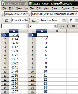
The code below reshapes these two vectors into a single two-column matrix (by columns, array constructors are in square brackets []), so in the final CSV file they represent two separate variables. Note that there is also an array constructor for two descriptive column names of the same string length.
! Here we save two huge integer vectors reshaping them into a single matrix
! by columns, see help on Fortran reshape function and array constructors.
! It also creates a vector of two column names for the output file.
call CSV_MATRIX_WRITE ( reshape(                                           &
                         [generation_one%individual%fitness,               &
                          generation_one%individual%person_number],        &
                         [POPSIZE, 2]),                                    &
                         "ZZZ1_all.csv",                                   &
                         ["FITNESS  ","ID_NUMBER"]                         &
                      )
So the resulting data CSV file is like this:
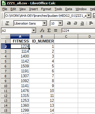
If the arrays to be combined have different types, it is possible to use whole-array type conversions to get some common type for all of the arrays. For example, if we combine an integer array A and a real array B (both having POPSIZE elements as above), it is wise to convert integer to real to avoid losing data precision:
! Here integer array A is converted to real so both A and B have the same type.
call CSV_MATRIX_WRITE ( reshape(                                           &
                         [real(A), B],                                     &
                         [POPSIZE, 2]),                                    &
                         "ZZZ1_all.csv",                                   &
                         ["FITNESS  ","ID_NUMBER"]                         &
                      )
We do not combine multiple loops manually, and automatic reshaping of the arrays is (usually) very fast.
8.14.4. Using an array of derived type containing arrays
The CSV_IO procedures do not directly work with derived types, only with simple arrays. Therefore, an interesting case is when one needs to save an array of a derived type, with a data component also being an array.
For example,
! Declare the derived type `struct_def`
type :: struct_def
  real, dimension(TYPE_MAX) :: array_comp
end type struct_def

! Declare an array of the objects of the type `struct_def`
type(struct_def), dimension(N_OBJECTS) :: objects_array
In this example, objects_array(:)%array_comp(:) is essentially a two dimensional matrix. But CSV module cannot work with derived type intrinsically. One needs to convert the derived type into a simple array.
The easiest way to do this is to define a temporary data array tmp_data that keeps data from the objects_array(:)%array_comp(:) data structure. Then, just save the tmp_data with CSV_MATRIX_WRITE.
! Convert the derived type components into a 2-D temporary array
do i = 1, N_OBJECTS
 do j=1, TYPE_MAX
   tmp_data(i,j) = objects_array(i)%array_comp(j)
 end do
end do

! Write the temporary array to the CSV output file.
call CSV_MATRIX_WRITE( tmp_data, "data_file.csv" )
Alternatively, conversion from the derived type arrays to simple array can be done inline through a combination of intrinsic reshape and implied loops:
! The derived type can be converted to the array inline by combination of
! reshape with two implied loops. This is a short version of the code.
call CSV_MATRIX_WRITE(                                                      &
    reshape( [( [( objects_array(i)%array_comp(j), i=1,N_OBJECTS )],        &
                                                        j=1, TYPE_MAX  )],  &
             [N_OBJECTS,TYPE_MAX] ),                                        &
    "data_file.csv"  )
8.15. Function: CSV_MATRIX_READ
This function reads a two-dimensional data matrix from a CSV or tab-separated data file. It has a single mandatory input parameter: the name of the file. The other optional parameters are: (1) output file read logical status (if TRUE then the file was successfully read); (2) input logical flag to include truncated records (default FALSE); (3) input real type missing code for substituting data in truncated and empty records.
Input parameters:
character (len=*) :: csv_file_name              ! File name to read.
logical           :: csv_file_status            ! Logical read success status.
logical           :: include_incomplete_records ! Flag to include truncated
                                                !  rows,  default FALSE.
real              :: missing_code               ! Code that substitutes data in
                                                !  truncated or empty records,
                                                !  if unset = -9999.0
Function value: an allocatable 2-dimensional real array.
real, dimension(:,:), allocatable :: matrix_out
|
|
CSV matrix subroutines use the "standard" arrangement for the matrix: the first index is for rows, the second, for columns. A reverse can be produced using the intrinsic transpose function. |
When reading the CSV file, the procedure excludes any lines that contain any non-numeric characters, therefore header line and text variable names are automatically excluded, only numeric values are read.
The function automatically allocates the output matrix, if file read operation was not successful (csv_file_status is FALSE), the output matrix dimensionality is (0,0). The number of rows (first dimension of the array) is determined as the total number of lines with all numeric characters, the number of columns is set from the first numeric line.
8.15.1. Truncated rows
If the read procedure encounters a row that contains a smaller number of numeric values than the first numeric row, it can substitute the missing data with specific missing data code (missing_code parameter, default -9999.0). To enable missing data substitution, the include_incomplete_records parameter should be TRUE.
"VAR1", "VAR2", "VAR3"
1.1,  1.2,  1.3
2.1,  2.2,  2.3
3.1,  3.2,  3.3
4.1,  4.2             ! <- truncated row
5.1,  5.2,  5.3
6.1                   ! <- truncated row
Default read mode:
Matr = CSV_MATRIX_READ(filename, errorflag)
The truncated rows (4.1, 4.2 and 6.1) are ignored in the output data:
1.1 |
1.2 |
1.3 |
2.1 |
2.2 |
2.3 |
3.1 |
3.2 |
3.3 |
5.1 |
5.2 |
5.3 |
Setting include_incomplete_records flag to TRUE
Matr = CSV_MATRIX_READ(filename, errorflag, .TRUE.)
makes the function read these truncated rows and append the missing data values with the missing data code:
1.1 |
1.2 |
1.3 |
2.1 |
2.2 |
2.3 |
3.1 |
3.2 |
3.3 |
4.1 |
4.2 |
-9999.0 |
5.1 |
5.2 |
5.3 |
6.1 |
-9999.0 |
-9999.0 |
A user provided missing data code would then result in such data:
Matr = CSV_MATRIX_READ(filename, errorflag, .TRUE., 100.0)
1.1 |
1.2 |
1.3 |
2.1 |
2.2 |
2.3 |
3.1 |
3.2 |
3.3 |
4.1 |
4.2 |
100.0 |
5.1 |
5.2 |
5.3 |
6.1 |
100.0 |
100.0 |
8.15.2. Real kind=8 data
It is possible to get a real kind=8 data matrix (double precision). To do this, the missing data code parameter should just have real(kind=8) type. The include_incomplete_data flag can be set to .FALSE., .TRUE. or absent (defaults to .FALSE.).
real (kind=8), dimension(:,:), allocatable :: Matr
....
Matr = CSV_MATRIX_READ( filename, errorflag, .FALSE., -9999.0_8 )
....
Matr = CSV_MATRIX_READ( filename, errorflag, -9999.0_8 )
....
Matr = CSV_MATRIX_READ( filename, errorflag, missing_code=100.0_8 )
8.16. Derived type: csv_file
This type is used as a unitary file handle object. It has the following structure:
type, public :: csv_file
  character (len=MAX_FILENAME) :: name  ! The name of the file
  integer :: unit = -1                  ! Fortran unit associated with the file
  logical :: status = .TRUE.            ! success flag for the latest operation
end type csv_file
If csv_file object is defined, the file name, unit and the latest operation success flag can be accessed as %name, %unit, %status (e.g. some_file%name, some_file%unit).
8.16.1. Basic Example
type(csv_file) :: file_occ              ! define the file handle object
....
file_occ%name="some_name.txt"           ! set file name value
....
call CSV_OPEN_WRITE(file_occ)           ! Open file for writing
....
call CSV_CLOSE(file_occ)                ! Close file
8.16.2. Arrays of structures
This derived type can be also used as an array. An example below shows how can this be done.
type(csv_file), dimension(:), allocatable :: file_ABM ! Define allocatable array
........                                              !   of file handle objects
allocate(file_ABM(modulators))                        ! Allocate this array
........
! now, use the array to handle many files of the same type
do j=1, modulators
  file_ABM(j)%name = "file_no_" // TOSTR(j,10) // ".csv"  ! Set file handle (j)
  call CSV_OPEN_WRITE(file_ABM(j))                        !   and use it
end do
|
|
The file name is set as a standard non-allocatable fixed string because allocatable strings may not be supported on all compiler types and versions. Notably, older GNU gfortran (prior to v.5) does not allow allocatable strings in derived types. Currently, MAX_FILENAME=255 (can be changed in the code). There is one consequence of using fixed strings: you may have to use the Fortran trim() function to cut off trailing blanks if strings are concatenated. E.g. do file_name=trim(String1) // trim(String2) instead of file_name=String1 // String2 or use file_name=CLEANUP(String1 // String2) to remove all blank and control characters. |
8.17. Extended example
Below is an extended example subroutine showing how to save diverse data to a CSV file. The example data variables come from an object oriented code, although the whole procedure does not use object orientation.
!> Save data for all agents within the population into a csv file.
subroutine population_save_data_all_agents_csv(this, output_data_file,      &
                                                    save_header, is_logging)
  use CSV_IO
  class(POPULATION), intent(in) :: this
  !> @param[in] output_data_file is the name of the CSV output file.
  character(len=*), intent(in) :: output_data_file
  !> @param[in] save_header turn ON/OFF of the descriptive file header.
  !!            Header is saved into the first row of the CSV output file
  !!            If not present, default is FALSE.
  logical, optional, intent(in) :: save_header
  !> @param[in] is_logging turn ON/OFF writing the file name and data into
  !!            the logger. If not present, default is TRUE.
  logical, optional, intent(in) :: is_logging

  ! Local copies of optionals.
  logical :: logging_enabled

  ! Counter
  integer :: ind

  !> ### Implementation notes ###
  !> #### Local variables for CSV backend ####
  !> - `N_COLUMNS` is the total number of columns in the spreadsheet data
  !!   file: it is equal to the number of variables that are saved for each
  !!   agent.
  integer, parameter :: N_COLUMNS = 21 ! equal to the number of columns
  !> - `handle_csv` is the CSV file handle object defining the file name,
  !!   Fortran unit and error descriptor, see HEDTOOLS manual for details.
  type(CSV_FILE) :: handle_csv
  !> - `csv_record_tmp` is the temporary character string that keeps the
  !!   whole record of the file, i.e. the whole row of the spreadsheet table.
  character(len=:), allocatable :: csv_record_tmp
  !> - `COLUMNS` is a parameter array that keeps all column headers; its
  !!   size is equal to the total number of variables (columns) in the data
  !!   spreadsheet file, which ic defined by the `N_COLUMNS` parameter here.
  !! .
  character(len=LABEL_LENGTH), dimension(N_COLUMNS),                        &
    parameter :: COLUMNS =  [ "ID_NUM   ", "PERS_NAME", "ALIVE    ",        &
                              "SEX_MALE ", "BODY_LEN ", "CTRL_RND ",        &
                              "BODY_MASS", "ENERGY   ", "STOMACH  ",        &
                              "MAXSTOMCP", "SMR      ", "HORM_GROW",        &
                              "HORM_THYR", "HORM_ADRE", "HORM_CORT",        &
                              "HORM_TEST", "HORM_ESTR", "N_REPROD ",        &
                              "N_OFFSPNG", "AGE      ", "FITNESS  "   ]

  ! PROCNAME is the procedure name for logging and debugging
  character(len=*), parameter ::                                            &
                          PROCNAME = "(population_save_data_all_agents_csv)"

  if (present(is_logging)) then
    logging_enabled = is_logging
  else
    logging_enabled = .TRUE.
  end if

  if (logging_enabled)                                                      &
    call LOG_MSG (LTAG_INFO // "Saving all individuals in population # " // &
            TOSTR(this%pop_number) // "(name '" // trim(this%pop_name) //   &
            "'), " //                                                       &
            "generation # " // TOSTR(Global_Generation_Number_Current) //   &
            ", time step " // TOSTR(Global_Time_Step_Model_Current) //      &
            " to file :" // output_data_file )

  !> #### Save data in CSV file ####
  !> - Define the file name \%name component of the CSV file handle. This
  !!   file handle object is now used as the sole file identifier.
  handle_csv%name = output_data_file
  !> - Open the output file defined by the `handle_csv` handle object for
  !!   writing.
  call CSV_OPEN_WRITE( handle_csv )

  !> - Possible error status of the latest file operation is obtained by the
  !!   \%status component of the file handle. Check if there were any errors
  !!   opening the file and report in the logger with the error tag.
  if ( .not. handle_csv%status ) then
      call LOG_MSG( LTAG_ERROR // "Opening output CSV file FAILED: " //     &
                    output_data_file // ", in " // PROCNAME )
      call LOG_MSG( LTAG_ERROR // "Data file " // output_data_file //       &
                    " is not written in " // PROCNAME )
      return
  end if

  !> - If the `save_header` flag is set to TRUE, save the CSV file header.
  if (present(save_header)) then
    if (save_header) call                                                   &
              CSV_HEADER_WRITE( "Population: " // this%pop_name, handle_csv )
  end if

  !> - Prepare the character string variable `csv_record_tmp` that keeps the
  !!   whole record (row) of data in the output CSV data file. The length of
  !!   this string should be enough to fit all the record data, otherwise
  !!   the record is truncated.
  csv_record_tmp = repeat(" ", N_COLUMNS * len(COLUMNS(1)) )

  !> - Produce the first record containing the column headers (variable
  !!   names). Note that `CSV_RECORD_APPEND()` accepts both arrays and scalar
  !!   values for appending. Also, write the first record physically to
  !!   the file.
  call CSV_RECORD_APPEND( csv_record_tmp, COLUMNS )
  call CSV_RECORD_WRITE ( csv_record_tmp, handle_csv )

  !> - The actual data are written to the CSV file in a loop over all the
  !!   individual members of the population. One record (row) of the data
  !!   file then represents a single individual.
  do ind = 1, size(this%individual)
    !>   - the `csv_record_tmp` character string variable is produced such
    !!     that it can fit the whole record;
    csv_record_tmp = repeat(" ",                                            &
                      max( CSV_GUESS_RECORD_LENGTH(N_COLUMNS+1,0.0_SRP),    &
                           len(this%individual(ind)%genome_label) ) )

    !>   - the actual data for the individual is appended to the current
    !!     record one by one. Note that logical values are converted to
    !!     integers using commondata::conv_l2r() function.
    associate ( AGENT => this%individual(ind) )
      call CSV_RECORD_APPEND(csv_record_tmp,AGENT%person_number        ) ! 1
      call CSV_RECORD_APPEND(csv_record_tmp,AGENT%genome_label         ) ! 2
      call CSV_RECORD_APPEND(csv_record_tmp,conv_l2r(AGENT%alive)      ) ! 3*
      call CSV_RECORD_APPEND(csv_record_tmp,conv_l2r(AGENT%sex_is_male)) ! 4*
      call CSV_RECORD_APPEND(csv_record_tmp,AGENT%body_length          ) ! 5
      call CSV_RECORD_APPEND(csv_record_tmp,AGENT%control_unselected   ) ! 6
      call CSV_RECORD_APPEND(csv_record_tmp,AGENT%body_mass            ) ! 7
      call CSV_RECORD_APPEND(csv_record_tmp,AGENT%energy_current       ) ! 8
      call CSV_RECORD_APPEND(csv_record_tmp,AGENT%stomach_content_mass ) ! 9
      call CSV_RECORD_APPEND(csv_record_tmp,AGENT%maxstomcap           ) ! 10
      call CSV_RECORD_APPEND(csv_record_tmp,AGENT%smr                  ) ! 11
      call CSV_RECORD_APPEND(csv_record_tmp,AGENT%growhorm_level       ) ! 12
      call CSV_RECORD_APPEND(csv_record_tmp,AGENT%thyroid_level        ) ! 13
      call CSV_RECORD_APPEND(csv_record_tmp,AGENT%adrenaline_level     ) ! 14
      call CSV_RECORD_APPEND(csv_record_tmp,AGENT%cortisol_level       ) ! 15
      call CSV_RECORD_APPEND(csv_record_tmp,AGENT%testosterone_level   ) ! 16
      call CSV_RECORD_APPEND(csv_record_tmp,AGENT%estrogen_level       ) ! 17
      call CSV_RECORD_APPEND(csv_record_tmp,AGENT%n_reproductions      ) ! 18
      call CSV_RECORD_APPEND(csv_record_tmp,AGENT%n_offspring          ) ! 19
      call CSV_RECORD_APPEND(csv_record_tmp,AGENT%age                  ) ! 20
      call CSV_RECORD_APPEND(csv_record_tmp,AGENT%fitness              ) ! 21
    end associate

    !>   - after all data are appended to the record, this record is
    !!     physically written to the disk using `CSV_RECORD_WRITE()`.
    !!   .
    call CSV_RECORD_WRITE( csv_record_tmp, handle_csv )

  end do

  !> - When all the records are saved, the CSV file is closed
  !!   with `CSV_CLOSE()`.
  call CSV_CLOSE( handle_csv )

  !> - This is finally sent to the logger (if `logging_enabled` is TRUE).
  !! .
  if (logging_enabled)                                                      &
    call LOG_MSG (LTAG_INFO // "Individual data saved, population size " // &
            TOSTR(this%population_size) //                                  &
            ", number of columns " // TOSTR(N_COLUMNS) )

end subroutine population_save_data_all_agents_csv
8.18. Procedures to manipulate the filesystem
There are several procedures for simple manipulations of the filesystem that are implemented as Fortran bindings to the standard POSIX C functions via Fortran interfaces.
The procedures have an optional parameter iostat for reporting the status of the operation. It retrns 0 in case of success and -1 if there was an error.
|
|
These subroutines might not work on all systems. However, tested and work on gfortran and ifort on both Linux and Windows and f95 (Oracle) on Linux. |
8.18.1. Subroutine: FS_MKDIR
Make a directory indicated by the first character string parameter (dirname). The second optional integer parameter iostat returns the error status of the operation, 0 in case of success, -1 if there was an error creating the directory.
Note that iostat error -1 is returned also if there is already a directory with the same name, so it might not be very informative practically.
The third, logical, optional parameter is_writeable can be used to check if the directory that has to be created is actually writeable. This parameter is useful, for example, in case when one needs to create a directory, but the directory happened to exist already (so iostat returns -1), although this is not a problem because the directory is still writeable (is_writeable returns TRUE).
dirname = "./model_output"
...
call FS_MKDIR(dirname, ierr) ! This checks the status if the mkdir itself.
....
call FS_MKDIR(dirname, is_writeable=success_write) ! This checks if the
                                                   ! directory is writeable.
8.18.2. Subroutine FS_RENAME
Rename a file.
call FS_RENAME("old_name", "new_name", i)
8.18.3. Subroutine FS_UNLINK
Deletes a file from the filesystem. Note that this subroutine does not delete directories for safety. Use FS_REMOVE subroutine for this.
call FS_UNLINK("obsolete_file", i)
8.18.4. Subroutine FS_REMOVE
Deletes a file or a directory from the filesystem.
call FS_REMOVE("delete_me", i)
8.18.5. Subroutine FS_CHDIR
Changes the current directory to a different one.
character(*), parameter :: output_folder = 'output'

....

call FS_CHDIR( output_folder )
Note: Note that call system("cd " // output_folder ) would not work because cd affects only the separate subshell created by system() command and does not pass to the calling Fortran program.
9. Module: BASE_RANDOM
This module contains subroutines for generating random numbers (pseudo-random number generator, PRNG). However, the code of this module depends on the platform and compiler used. The build system (make) generates the appropriate header file automatically.
9.1. Subroutine: RANDOM_SEED_INIT
Initialise the random seed for random number generation. This module uses an improved random seed generation algorithm that uses the system entropy pool on Unix systems and XOR of the current time and PID on Windows. Therefore, it is safe for use on parallel processing systems. Normally has no parameters.
call RANDOM_SEED_INIT()
RANDOM_SEED_INIT can optionally return the current (calculated) seed as two parameters: integer dimension of the seed array n_here and the array itself seed_here. This, however, is useful only for debugging.
integer :: dbg_seed_size                      ! depends on compiler/platform
integer, dimension (12) :: dbg_seed_array     ! ... can be 12 or 2 on x86
...
call RANDOM_SEED_INIT(dbg_seed_size, dbg_seed_array)
print *, "Seed: ", dbg_seed_size, ", array: ", dbg_seed_array(:dbg_seed_size)
The seed array size can be different: on GNU gfortran x86 it is 12, on Intel and Oracle Fortran (both x86) it is 2.
9.2. Function: RAND_I
Generates a random integer (uniform distribution) within the range A to B (the two parameters of the function).
ipos = RAND_I(1, len(ga_target))
9.3. Functions: RAND_R4 (RAND) and RAND_R8
Generates a random real (kind 4 or 8) number with the uniform distribution. If the function has no parameters, it calculates a uniform random number ranging from 0 to 1. May have two real or integer parameters defining the desired range (minimum, maximum) of the random numbers. RAND is an alias for RAND_R4.
if ( RAND() < ga_mutationrate ) then
  call mutate(fish(i))
end if
.....
rate = RAND_R4(10,100) ! this generates a random number within 10..100
|
|
These functions are just wrappers to the standard Fortran subroutine random_number. Note that such intrinsic Fortran functions as RAN are provided for backwards compatibility with the old Fortran 77 standard. They are usually implemented as a simple modulo generator (as in f77). The new standard random_number implements a superior algorithm and should be used for all new codes. |
9.4. Functions: RNORM_R4, RNORM_R8, RNORM
In absence of any parameters, RNORM generates a normally distributed real (kind 4) random number with zero mean and standard deviation = 1.0. May also have two real parameters defining the desired mean and variance. RNORM_R4 forces 32 bit real (kind 4) while RNORM_R8 does 64 bit (kind 8).
Based on algorithm 712, Transactions on Mathematical Software, 18, 4, 434-435 (1992); (Kinderman & Monahan, augmented with quadratic bounding curves).
ga_mut  = RNORM()             ! generate Gaussian variate with mean 0 and variance 1
ga_len  = RNORM(100.,10.)     ! generate Gaussian variate with mean 100 and variance 10
ga_len8 = RNORM(100._8,10._8) ! same as previous but kind 8 (double precision)
9.5. Function: RAND_STRING
Generates a string composed of random characters. It has a single mandatory integer parameter, the string length. There are also two optional integer parameters defining the range of the ASCII character codes for this string.
Some useful ranges: numbers 48:122, Latin alphanumeric characters 65:122, uppercase Latin letters 65:90, lowercase Latin letters: 97:122.
LABEL = RAND_STRING(24,97,122) ! Set a random label of 24 lowercase letters
9.6. Arrays of random numbers: RAND_ARRAY and RNORM_ARRAY
The subroutines RAND_ARRAY and RNORM_ARRAY generate arrays (up to 6-dimensions) of uniform and normal (Gaussian) random numbers, respectively. RAND_ARRAY can generate real (kind=4 or 8) and integer arrays. In absence of additional parameters, RAND_ARRAY produces values ranging within 0.0 and 1.0, RNORM_ARRAY, normal (Gaussian) values with zero mean and unity standard deviation.
Additional parameters for arbitrary random numbers. As with the above single-value functions, additional parameters enable the generation of random numbers with arbitrary parameters. For example, two additional parameters of RAND_ARRAY define the range (minimum, maximum) of uniformly distributed numbers whereas two additional parameters of RNORM_ARRAY determines the mean and variance of the Gaussian random numbers generated.
The subroutine RAND_ARRAY can be also used with an integer array as a parameter. In this case, the subroutine requires two additional mandatory integer parameters that set the range of the integers generated.
There are aliases RAND_MATRIX and RNORM_MATRIX for two- to six-dimensional matrices.
Here are a few examples:
real, dimension(200,500)  :: ARRAY_X, ARRAY_Y, ARRAY_Z
integer, dimension(20,20) :: ARRAY_I
....
call RAND_ARRAY(ARRAY_X)         ! produce 2D array of uniform random numbers
...
call RAND_ARRAY(ARRAY_X,10.,20.) ! produce 2D array of uniform random numbers
                                 !   ranging from 10.0 to 20.0
...
call RNORM_ARRAY(ARRAY_Y)        ! produce 2D array of random normal variates
                                 !   (mean=0, std.dev.=1)
...
call RNORM_MATRIX(ARRAY_Z,1.,.2) ! produce 2D array of Gaussian numbers with
                                 !   mean=1.0 and variance=0.2
...
call RAND_ARRAY(ARRAY_I,1,10)    ! produce 2D array of integers ranging 1 to 10
9.7. Random permutation: PERMUTE_RANDOM function
PERMUTE_RANDOM produces a random permutation index array, i.e. an array of integers from 1 to N in a randomised order. It takes a single integer argument, the size of the random permutation index array (N).
print *, PERMUTE_RANDOM(10)         ! Produces:  7, 4, 5, 10, 3, 9, 2, 1, 8, 6
print *, X(PERMUTE_RANDOM(size(X))) ! Elements of the array X in random order
9.8. Usage Notes
If the parameter type is ambiguous while calling the PRNG function, "single precision" (kind 4) is used by default. For example, the following involves type conversion from kind 4 to kind 8:
real(8) :: ga_mut   ! kind 8 type real
...
ga_mut  = RNORM()   ! RNORM returns a kind 4 value, assigned to kind 8 variable
Be careful when using literal constants as parameters. They should normally have the same type as the main argument. For example, numerical parameters in the example below should be explicitly kind 8, otherwise this error will be issued: "There is no specific subroutine for the generic rnorm_array."
real(8), dimension(ROWS)      :: C  ! declarations use kid 8
real(8), dimension(ROWS,COLS) :: D
....
call RAND_ARRAY(C, 10._8,25._8)     ! correct call as all arguments are kind 8
call RNORM_ARRAY(D, 10._8, 25._8)
....
call RAND_ARRAY(C, 10, 25)          ! compiler error, type mismatch, not kind 8
call RNORM_ARRAY(D, 10., 25.)
(This limitation might change in future if mixed type functions are implemented.)
9.9. Build details
When not using the automatic build system based on GNU make, the module subroutine RANDOM_SEED_INIT should be tweaked according to the compiler and platform as follows:
GNU fortran:
!*****************************************************************************
! *** NON-PORTABLE CODE BEGIN ***

use ISO_FORTRAN_ENV, only: int64   ! GNU and Intel

implicit none

integer, allocatable :: seed(:)
integer :: i, n, un, istat, dt(8), pid
integer(int64) :: t

! *** NON-PORTABLE CODE END ***
!*****************************************************************************
Intel Fortran
!*****************************************************************************
! *** NON-PORTABLE CODE BEGIN ***

use ISO_FORTRAN_ENV, only: int64  ! GNU and Intel

use IFPORT, only : getpid         ! getpid is an extension defined in IFPORT

implicit none

integer, allocatable :: seed(:)
integer :: i, n, un, istat, dt(8), pid
integer(int64) :: t

! *** NON-PORTABLE CODE END ***
!*****************************************************************************
Oracle Fortran
!*****************************************************************************
! *** NON-PORTABLE CODE BEGIN ***

! External Modules not used on Oracle f95, but an include header must be placed

implicit none

integer, allocatable :: seed(:)
integer :: i, n, un, istat, dt(8), pid
integer, parameter :: int64 = selected_int_kind(18) ! define int64
integer(int64) :: t

include "system.inc"  ! Include non-intrinsic library headers for the Oracle f95

! *** NON-PORTABLE CODE END ***
!*****************************************************************************
The build system based on GNU make does this automatically.
10. Module: LOGGER
10.1. Overview
This module controls logging arbitrary messages during the execution of the program. The format and destination of the messages is configurable during the run time. Thus, a trace of the execution can be read by the user during and after the execution. The module includes subroutines to connect a file to the logger, configure the logging process, for example enable or disable the terminal (stdout) messages, issue actual log messages. There are four log levels (volume, chapter, section and subsection) that can differ a little in the visual representation, it can be useful for marking specific parts of the log. Logging is especially useful for simulation models that run for quite a long time like AHA. The user can then check the log from time to time to make sure everything is in order and get an idea about where it is running now.
Here is an example of a log file with timestamps (date and time printed on the left of the log strings) being displayed using the Follow program.
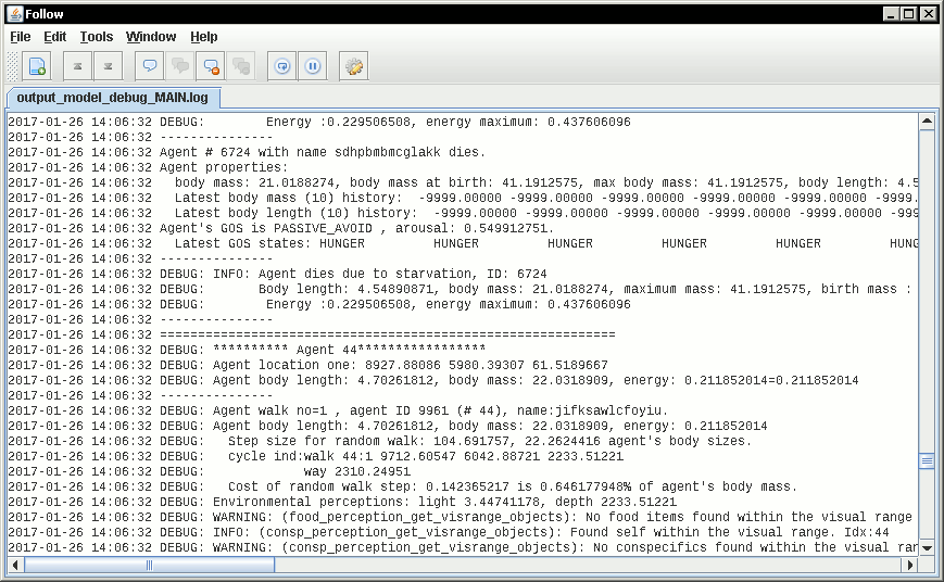
10.2. Subroutine: LOG_STARTUP
The logger must be started up with the subroutine LOG_STARTUP that has the log file name as a parameter, for example call LOG_STARTUP("logfile-01.log"). The second optional argument defines if the existing log file with the same name should be appended (.TRUE., default) or overwritten (.FALSE.). The code below shows how to start logging and build the log file from parts:
!> Set log file name from string parts and start logging, *overwrite* old log
call LOG_STARTUP("output_" // MODEL_NAME // "_" // TAG_MMDD() // &
                 "_MAIN.log", .FALSE.)
10.3. Subroutine: LOG_CONFIGURE
There are also several configuration options for the LOGGER which are called using the LOG_CONFIGURE subroutine.
LOG_CONFIGURE accepts two parameters:
-
character string parameter name
-
parameter value (character string, integer or logical type)
These are the possible configuration options and their explanations:
| Option | Value | Explanation |
|---|---|---|
timestamp |
logical TRUE/FALSE |
if timestamp is issued in the log |
writeonstdout |
logical TRUE/FALSE |
if the log should also go to terminal (stdout) |
writeonlogfile |
logical TRUE/FALSE |
if the log should also go to the disk file |
stoponerror |
logical TRUE/FALSE |
defines if execution should stop on error |
logfileunit |
integer value |
Set specific unit for log (use with caution!) |
level_string_volume |
string delimiter |
Set the string for volume |
level_string_chapter |
string delimiter |
Set the string for chapter |
level_string_section |
string delimiter |
Set the string for section |
level_string_subsection |
string delimiter |
Set the string for subsection |
The following code shows an example of LOGGER configuration. Here it turns on printing timestamps in the log and chooses whether log messages should also go to the screen terminal (stdout).
call LOG_CONFIGURE("timestamp", .TRUE.)         ! do timestamps in the log

if (IS_DEBUG) then
  call LOG_CONFIGURE("writeonstdout" , .TRUE.)  ! output also to screen if DEBUG
else
  call LOG_CONFIGURE("writeonstdout" , .FALSE.) ! NO screen log output normally
end if
10.4. Function: LOG_ISINITIALIZED
The logical function LOG_ISINITIALIZED returns TRUE if the logger is already initialised.
if (LOG_ISINITIALIZED) then
10.5. Subroutine: LOG_CGET
The subroutine LOG_CGET is used to query a LOGGER configuration option value. It has two parameters, character string option and logical, integer or character string value. Its use is similar to LOG_CONFIGURE.
call LOG_CGET("writeonstdout", is_stdout) ! check if log is going to screen
10.6. Subroutine: LOG_DELIMITER
LOG_DELIMITER issues a string delimiter to the log, it has an optional integer argument setting the kind of the delimiter, default is "volume" (1). This is useful to mark the log with visually different parts. The maximum string length of the delimiter is 80 characters (set as a public integer parameter LOG_LEVEL_DELIMITER_LENGTH).
The four levels of logging volume, chapter, section and subsection are defined in the module LOGGER as constants, so these constant can be used instead of the integer number. There are also the default delimiter strings.
integer , parameter , public :: LOG_LEVEL_VOLUME = 1      ! "==============="
integer , parameter , public :: LOG_LEVEL_CHAPTER = 2     ! "---------------"
integer , parameter , public :: LOG_LEVEL_SECTION = 3     ! "***************"
integer , parameter , public :: LOG_LEVEL_SUBSECTION = 4  ! "+++++++++++++++"
Below is a code example of issuing log delimiters:
call LOG_DELIMITER(1)                     ! issues volume     "---------------"
.....
call LOG_DELIMITER(LOG_LEVEL_SUBSECTION)  ! issues subsection "+++++++++++++++"
Using a user-defined delimiter string is illustrated below.
! Set delimiter as a 60-characters long line of "======..." for volume delimiter
call LOG_CONFIGURE("level_string_volume", repeat("=",60))
.......
call LOG_DELIMITER(LOG_LEVEL_VOLUME)      ! issues this long delimiter line
10.7. Subroutine: LOG_SHUTDOWN
LOG_SHUTDOWN: The last thing to do is to shut down logging with the LOG_SHUTDOWN subroutine:
call LOG_SHUTDOWN () ! close logger
11. Module: BASE_STRINGS
This module containing some useful string manipulation functions is borrowed from http://www.gbenthien.net/strings/index.html. The description below is just repeating the official doc file included with the module. Note that there are a couple of utils (GETFLINE, WRITEQ) in this module that work with files. These use the standard Fortran unit to refer for the file and unlike the other modules here are not adjusted (yet) to use the file handle object (csv_file).
|
|
These utilities are currently provided "as is," not well tested, contain unsafe code and probably some bugs. |
One issue is that they do not work with strings declared as parameters
[They do not explicitly use intent.]
For example, this code does
work as expected:
character(len=40) :: st_inp = "AAA BBB CCC*DDD"           ! normal string
character(len=6), dimension(6) :: st_out
call parse(st_inp, " *", st_out, i)
Whereas this (st_inp is a parameter) results in invalid memory reference:
character(len=*), parameter :: st_inp = "AAA BBB CCC*DDD" ! fixed parameter
character(len=6), dimension(6) :: st_out
call parse(st_inp, " *", st_out, i)
SB: I shall recode and fix them if and when I have time, but the priority is low.
Fortran Character String Utilities. A collection of string manipulation routines is contained in the module ‘strings’ found in the file stringmod.f90. To obtain this module as well as some other string utilities, go to the website http://www.gbenthien.net/strings/index.html. To use the routines in the module ‘strings’ the user needs to add the statement use strings to the top of the program. These routines were developed primarily to aid in the reading and manipulation of input data from an ASCII text file. The routines are described below.
11.1. Subroutine: PARSE
SUBROUTINE PARSE(str, delims, args, nargs)
This routine was originally designed to separate the arguments in a command line where the arguments are separated by certain delimiters (commas, spaces, etc.). However, this routine can be used to separate other types of strings into their component parts. The first input is a string str (e.g., a command line). The second argument is a string delims containing the allowed delimiters. For example, delims might be the string " ," consisting of a comma and a space. The third argument is a character array args that contains on output the substrings (arguments) separated by the delimiters. Initial spaces in the substrings (arguments) are deleted. The final argument is an integer nargs that gives the number of separated parts (arguments). To treat a delimiter in str as an ordinary character precede it by a backslash (\). If a backslash character is desired in str, precede it by another backslash (\\). In addition, spaces that immediately precede or follow another delimiter are not considered delimiters. Multiple spaces or tabs are considered as a single space, i.e., "a b" is treated the same as "a b". Backslashes can be removed from an argument by calling the routine REMOVEBKSL, i.e.,
call REMOVEBKSL(<string>)
This routine converts double backslashes (\\) to single backslashes (\).
Example: If the delimiters are a comma and a space (delims = " ,"), then the subroutine PARSE applied to the string "cmd arg1 arg\ 2 arg3" produces the output:
args(1) = cmd
args(2) = arg1
args(3) = arg 2
args(4) = arg3
nargs = 4
11.2. Subroutine: COMPACT
SUBROUTINE COMPACT(str)
This routine converts multiple spaces and tabs to single spaces and deletes control characters.
11.3. Subroutine: REMOVESP
SUBROUTINE REMOVESP(str)
This routine removes spaces, tabs, and control characters in string str.
11.4. Subroutine: OUTSTRIP
SUBROUTINE OUTSTRIP(str, set)
This subroutine removes all characters in the set set from the string str:
call OUTSTRIP(name_sys, ":,.:") ! remove punctuation from name_sys
11.5. Subroutine: VALUE
SUBROUTINE VALUE(str, number, ios)
This subroutine converts a number string to a number. The argument str is a string representing a number. The argument number is the resulting real number or integer (single or double precision). The argument ios is an error flag. If ios is nonzero, then there was an error in the conversion.
11.6. Subroutine: SHIFTSTR
SUBROUTINE SHIFTSTR(str, n)
This routine shifts characters in the string str by n positions (positive values denote a right shift and negative values denote a left shift). Characters that are shifted off the end are lost. Positions opened up by the shift are replaced by spaces.
11.7. Subroutine: INSERTSTR
SUBROUTINE INSERTSTR(str, strins, loc)
This routine inserts the string strins into the string str at position loc. Characters in str starting at position loc are shifted right to make room for the inserted string.
11.8. Subroutine: DELSUBSTR
SUBROUTINE DELSUBSTR(str, substr)
This subroutine deletes the first occurrence of substring substr from string str and shifts characters left to fill hole.
11.9. Subroutine: DELALL
SUBROUTINE DELALL(str, substr)
This routine deletes all occurrences of substring substr from string str and shifts characters left to fill holes.
11.10. Function: UPPERCASE
FUNCTION UPPERCASE(str)
This function returns a string that is like the string str with all characters that are not between a pair of quotes (" " or ' ') converted to uppercase.
11.11. Function: LOWERCASE
FUNCTION LOWERCASE(str)
This function returns a string that is like the string str with all characters that are not between a pair of quotes (" " or ' ') converted to lowercase.
11.12. Subroutine: GETFLINE
SUBROUTINE GETFLINE(nunitr, line, ios)
This routine reads a line from unit nunitr, ignoring blank lines and deleting comments beginning with an exclamation point(!). The line is placed in the string line. The argument ios is an error flag. If ios is not equal to zero, then there has been an error in the read operation. A negative value for ios denotes an end of file.
|
|
There is a more powerful function READLINE in CSV_IO. |
11.13. Function: MATCH
FUNCTION MATCH(str, ipos)
This function returns the delimiter in string str that matches the delimiter in position ipos of str. The output is the position of the matching delimiter or -1 in case of error (e.g. no matching delimiter). Allowable delimiters are (), [], {}, <>.
11.14. Subroutine: WRITENUM
SUBROUTINE WRITENUM(number, string, fmt)
This routine writes a number to a string. The argument number is a real number or an integer (single or double precision). The number number is written to the character string string with format fmt (e.g., "e15.6" or "i5").
11.15. Subroutine: TRIMZERO
SUBROUTINE TRIMZERO(str)
This subroutine deletes nonsignificant trailing zeroes in a number string str. A single zero following a decimal point is allowed. For example, "1.50000" is converted to "1.5" and "5." is converted to "5.0".
11.16. Subroutine: WRITEQ
SUBROUTINE WRITEQ(unit, name, value, fmt)
This routine writes a string of the form "name=value" to the unit unit. Here name is the input string name and value is the input number value converted to a string with the format fmt. The number value can be a real number or an integer (single or double precision).
11.17. Function: IS_LETTER
FUNCTION IS_LETTER(ch)
This function returns the logical value .TRUE. if the input character ch is a letter (a–z or A–Z). It returns the value .FALSE. otherwise.
11.18. Function: IS_DIGIT
FUNCTION IS_DIGIT(ch)
This function returns the logical value .TRUE. if the input character ch is a digit (0–9). It returns the value .FALSE. otherwise.
11.19. Subroutine: SPLIT
SUBROUTINE SPLIT(str, delims, before, sep)
This routine uses the first occurrence of a character from the string delims in the string str to split the string into two parts. The portion of str before the found delimiter is output in before; the portion of str after the found delimiter is output in str (str is left justified). The output character sep (optional) contains the found delimiter. To treat a delimiter in str as an ordinary character precede it by a backslash (\). If a backslash is desired in str, precede it by another backslash (\\). Repeated applications of SPLIT can be used to parse a string into its component parts. Backslashes can be removed by calling the routine REMOVEBKSL, i.e., call REMOVEBKSL(string)
12. IEEE Arithmetics
12.1. Overview
The model can now use the IEEE arithmetic modules. They allow exact control of the CPU math features and exceptions caused by invalid calculations, such as dividion by zero, overflow, underflow etc. A potential issue is that they have an optional status in the Fortran standard, so compilers do not have to implement them, although many do.
|
|
IEEE arithmetic and exceptions are fully described in chapter 14 of this book: Adams, et al., 2009 The Fortran 2003 Handbook. Springer. |
For example, Intel Fortran implements intrinsic IEEE arithmetics
modules. GNU Fortran does not implement them untile version 5.
[It was
because GNU compiler collection is made for portability and supports many
different processor architectures in addition to the most common x86 and
implementation of IEEE modules is highly dependent on the CPU type and
features.]
However, there are external (non-intrinsic) IEEE modules for gfortran
on the x86 (support both 32 and 64 bit) that are included into the HEDTOOLS
bundle.
|
|
the fimm HPC cluster, where calculations are normally performed, has GNU Fortran 4.8.1 and will require non-intrinsic IEEE modules. It also has the Intel Fortran which has built-in (intrinsic) IEEE modules though. |
12.2. IEEE Exceptions
There are several exception conditions:
-
IEEE_DIVIDE_BY_ZERO
-
IEEE_INEXACT
-
IEEE_INVALID
-
IEEE_OVERFLOW
-
IEEE_UNDERFLOW
-
IEEE_USUAL (An array of three exceptions IEEE_OVERFLOW, IEEE_DIVIDE_BY_ZERO, IEEE_INVALID)
-
IEEE_ALL (An array of five exceptions IEEE_OVERFLOW,IEEE_DIVIDE_BY_ZERO, IEEE_INVALID, IEEE_UNDERFLOW, IEEE_INEXACT)
Normally, if the program encounters invalid arithmetic calculations, then it
should crash or at least report the problem. Otherwise, correctness of
calculations is not guaranteed. By default, many compilers just ignore invalid
calculations (even many cases of division by zero, NaN
["Not a Number,"
a wrong arithmetic value that is not equal to itself, can result from many math
errors]
generation etc.).
In most cases NaNs and other invalid arithmetics strongly point to a bug. If a NaN value is just left ignored during the calculations, it will likely propagate further into some other calculations making them invalid. It is therefore wise to turn halting ON by default in model calculations (unlike normal utility software that should never crash).
Turning arithmetic exception halting ON during the compile time requires specific compiler options.
| Compiler | option | example |
|---|---|---|
GNU GCC |
-ffpe-trap |
-ffpe-trap=zero,invalid,overflow,underflow |
Intel Fortran |
-fpe (/fpe) |
-fpe0 (/fpe:0 on Windows) |
Solaris Studio |
--ftrap |
--ftrap=invalid,overflow,division |
The IEEE module IEEE_EXCEPTIONS allows to control halting during the run time. For example, it is cool to switch halting ON in specific troublesome parts of the code that can normally result in invalid calculations (division by zero, invalid, inexact etc.) and control each such occurrence specifically (e.g. provide a subroutine handling and fixing the calculations).
Halting the program that encounters specific condition is controlled via IEEE_GET_HALTING_MODE subroutine (returns logical parameter IEEE_DEF_MODE). For example, for IEEE_INVALID it is:
call IEEE_GET_HALTING_MODE(IEEE_INVALID, IEEE_DEF_MODE)
It is also possible to set specific halting mode for specific condition. For example, to set halting ON (execution termination) on invalid arithmetic do this:
call IEEE_SET_HALTING_MODE(IEEE_INVALID, .TRUE.) ! Will halt on IEEE_INVALID
Here is an example:
...
! Invoke IEEE Arithmetics:
! use, non_intrinsic :: IEEE_EXCEPTIONS ! if gfortran v<5

! We normally use included auto-generated wrapper for the module
include "IEEE_wrap.inc"

IMPLICIT NONE

REAL    r,c,C0,Ap,Vc,Ke,Eb
REAL    FR1,FR2,F1,FDER

....

logical :: IEEE_MATH_FLAG, IEEE_DEF_MODE  ! values for IEEE math modules

call IEEE_GET_HALTING_MODE(IEEE_INVALID, IEEE_DEF_MODE) ! Get default halting
call IEEE_SET_HALTING_MODE(IEEE_INVALID, .FALSE.)       ! NO halting from here!

...

FR2=LOG(ABS(C0)*Ap*Vc)
FR1=LOG(((Ke+Eb)/Eb)*r*r*EXP(c*r))
F1 = FR1-FR2
FDER = c + 2./r

call IEEE_GET_FLAG(IEEE_INVALID, IEEE_MATH_FLAG) ! Get the error flag
if(IEEE_MATH_FLAG) then
  ! if IEEE exception is signalled, we cannot relay on the calculations
  ! Report the error: remember there is no halting now, the program won't stop
  write(10,*) "IEEE exception in DERIV ", r,F1,FDER,c,C0,Ap,Vc,Ke,Eb
  ! We also have to fix the calculations, e.g. equate some values to zero
  r=0.; F1=0.; FDER=0.
  call IEEE_SET_FLAG(IEEE_INVALID, .FALSE.) ! Set the error flag back to FALSE
end if

...

call IEEE_SET_HALTING_MODE(IEEE_INVALID, IEEE_DEF_MODE) ! Set default halting

END SUBROUTINE DERIV
12.3. Implementation details
We use an automatic build system (see below) which normally keeps track of the compiler and its version and IEEE modules support, there is no need to include use, intrinsic (or non_intrinsic) :: IEEE_EXCEPTIONS and tweak it manually depending on the compiler support. The build system automatically generates the correct include file IEEE_wrap.inc which should be inserted into the code in place of use … statement:
SUBROUTINE DERIV(r,F1,FDER,c,C0,Ap,Vc,Ke,Eb)
!Derivation of equation for visual range of a predator

! Invoke IEEE Arithmetics:
! use, non_intrinsic :: IEEE_EXCEPTIONS ! if gfortran v<5

! We normally use included auto-generated wrapper for the module
include "IEEE_wrap.inc"

REAL    r,c,C0,Ap,Vc,Ke,Eb
....
Without the GNU make-based build system, the rule is simple. Use
non-intrinsic modules with GNU gfortran version <5.0
[e.g. gfortran
on the fimm cluster]
and build the modules beforehand:
!*****************************************************************************
! *** NON-PORTABLE CODE BEGIN ***
use, non_intrinsic :: IEEE_FEATURES
use, non_intrinsic :: IEEE_ARITHMETIC
use, non_intrinsic :: IEEE_EXCEPTIONS
! *** NON-PORTABLE CODE END ***
!*****************************************************************************
and intrinsic modules on GNU gfortran v>5, Intel Fortran or Oracle Fortran:
!*****************************************************************************
! *** NON-PORTABLE CODE BEGIN ***
use, intrinsic :: IEEE_FEATURES
use, intrinsic :: IEEE_ARITHMETIC
use, intrinsic :: IEEE_EXCEPTIONS
! *** NON-PORTABLE CODE END ***
!*****************************************************************************
13. Build system: GNU make
13.1. Overview
The model currently uses a build system based on GNU make (Makefile). GNU make is an automated system for building source code (in fact, any digital project that requires keeping track of dependencies between multiple components.)
— Mecklenburg R.
All the build rules for building the model executable are collected in the Makefile. If the model requires external components (e.g. non-intrinsic IEEE math modules), they will be automatically inserted.
GNU make is good because it works on diverse combinations of platforms and OSs (e.g. Linux and Windows). Some proprietary Unix platforms could supply the vendor’s make utility that may not be compatible with the GNU make (e.g. Oracle Solaris includes its own make clone). There might be an option turning on GNU compatibility. But it is better to use the GNU make (gmake on Solaris) anyway.
|
|
A good manual on the GNU Make is this book: Mecklenburg, R, 2005, Managing Projects with GNU Make, Third edition. O’Reilly. There is also the official GNU Make Manual. |
13.2. Using make
Most basic things with the standard Makefile are simple. The commands are issued on the terminal console.
|
|
There is a separate Makefile in the HEDTOOLS bundle. It is used for building the modelling tools as a static library. Separate building of HEDTOOLS is normally not necessary. Just tweak and run the Makefile that is supplied in the current model directory. It will build HEDTOOLS and, if necessary, IEEE modules automatically. |
The make system keeps track of all the code components. For example, if only one has been changed, it will recompile only this. It also keeps track of whether IEEE math modules are really necessary and if the intrinsic or non-intrinsic modules are used.
For example, you may have built the model executable (make) and then edited the code of a module a little. Then just issue command to run batch (make run) on fimm. The make system will then automatically determine that the model executable is now out of date and recompile the changed module and build an updated executable, and only after this will start the batch job.
Another example: you just checked-out or updated (e.g. svn up) the model source that is tested and known to be bug-free on the fimm cluster. Now you should compile components of the program, (e.g. tweak IEEE math modules), build the executable, and finally start the executable in the cluster’s batch job system. All this is done using a single command: make run.
$ svn update
$ ... some output...
$ make run
The system should work the same way on Windows, Mac and Linux including the fimm HPC cluster. By editing the Makefile provided, one can easily tweak the behaviour of the build process, e.g. add other modules, change names, compilation options and details etc.
Microsoft Studio, Oracle Solaris Studio and other similar IDEs actually provide their own make systems (e.g. nmake, make or dmake) that work behind the scenes even if the IDE GUI is used.
|
|
The HEDTOOLS bundle has a subdirectory called template that contains a template Makefile for new modelling projects. In many cases only the source code file name(s) have to be tweaked there. |
13.2.1. Building and running the model
-
Get a short help on the options: make help
-
Autogenerate model documentation with Doxygen: make docs
-
Build the model executable using default compiler: make
-
Force rebuild the model executable with Intel compiler: make intel
-
Force rebuild the model executable with GNU compiler: make gnu
-
Run the current model: make run (on the fimm HPC cluster, this will automatically start a new batch job)
|
|
On some systems, running the AHA Model compiled with the Intel Fortran compiler crashes with "stack overflow"" or "segmentation fault". This is because of the model can have large number of concurrent threads working with large data arrays. To fix it on Linux, issue this command: ulimit -s unlimited on the terminal. The same error on Windows is corrected by increasing stack size with the /F100000000 ifort compiler option (this is normally already fixed in the Makefile). Increasing stack size on Mac OS X is described here. |
13.2.2. Cleanup
There are also a few options for deteting the files and data generated by the build process.
-
Remove all the data generated by the model make cleandata
-
Remove all the data files generated by the model run as well as the model executable: make clean
-
Remove everything generated by the build system and all the data, retain the default state: make distclean
|
|
If there are weird build errors, like cannot find logger.mod while the module is in fact there, use make distclean for a complete cleanup first and then issue normal make again. |
13.2.3. Debugging
The environment variable DEBUG controls whether the build system produces the debug symbols (-g) or, if NOT defined, speed-optimised machine code (-O3, automatic loop parallelization etc.). To build with debug support just define DEBUG in the manner standard for the platform/OS. For example, on Linux use:
$ DEBUG=1 make
or (DEBUG is now persistent)
$ export DEBUG=1
$ make
on Windows:
O:\WORK\MODEL\HED18>set DEBUG=1
O:\WORK\MODEL\HED18>make
or use DEBUG as a parameter to make, this works on all platforms:
$ make intel DEBUG=1
13.2.4. Profiling
Building the model code for profiling using the GNU toolset is similar to debugging. Here the variable PROFILE is used the same way.
$ PROFILE=1 make
Running the program that has been built with profiling enabled will generate a profiling report: gmon.out that contains various execution timing statistics. This report can be read and analysed with the gprof utility, for example:
$ gprof MODEL.exe
|
|
Profiling currently works only with the GNU toolset (GNU gfortran and GNU profiler). |
13.2.5. Compiling documentation
Doxygen documentation for the model (extracted from the source code comments) is produced using this command:
make docs
Additionally, this document can be compiled in the HEDTOOLS directory with:
make doc
|
|
Note doc not docs as in the model Doxygen documentation. |
The default output format for this manual is PDF. Any other format supported by asciidoc can be produced by setting the DOCFMT variable. For example, Epub is compiled using:
make doc DOCFMT=epub
|
|
Compiling this document in PDF and other supported output formats requires the asciidoc markup processor. Asciidoc is not required for anything else. |
13.2.6. Using Intel Parallel Studio on Windows (command line)
Using Makefile with the Intel Parallel Studio XE 2013 Fortran compiler (ifort.exe) (and probably other versions of Intel Fortran on Windows) requires setting up the Microsoft Studio environment. This is normally done by calling the Command Prompt from the menu:
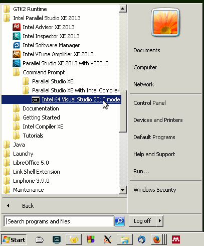
Or if you right click on the shortcut, copy the commend line set in the menu and run it in the terminal. Such a command may look like this:
C:\Windows\SysWOW64\cmd.exe /E:ON /V:ON /K ""C:\Program Files (x86)\Intel\Composer XE 2013\bin\ipsxe-comp-vars.bat" intel64 vs2010"
Then running this command will result in this:
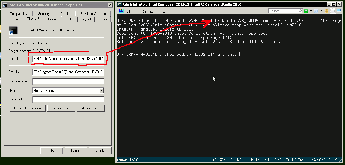
Once the Intel command prompt environment is set, we can use the make command as normal with the Intel Fortran compiler, e.g. build using the Intel ifort on Windows:
make intel
|
|
It is crucial to set up the Intel Fortran command prompt build environment on the Windows platform, otherwise make would not find all the necessary Intel Parallel Studio and Microsoft Studio compiler and linker components. This is not necessary on the Linux Intel Fortran compiler. |
If you use the ConEmu terminal, the command to set up the Intel Parallel Studio environment can be inserted in the ConEmu startup command line or script.
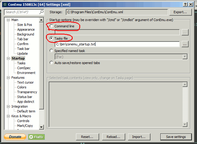
In the simplest case, the Startup command line or startup script might contain something like this (note that it is a single line with commands separated by ampersands &):
cmd.exe /C call "C:\Program Files (x86)\Intel\Composer XE 2013\bin\ipsxe-comp-vars.bat" intel64 vs2010 & "C:\Program Files\Far Manager\far.exe"
The exact path to the ipsxe-comp-vars.bat should be taken from the menu shortcut. In the above case, ConEmu will call the command prompt setup batch script ipsxe-comp-vars.bat (with full path and platform parameters intel64 vs2010) and then run the Far Manager (also full path is here).
If you like to use different tasks in ConEmu, such initialisation command, tweaked for particular task can be also inserted the Startup → Tasks → Commands menu; here is an almost identical example calling Far Manager:
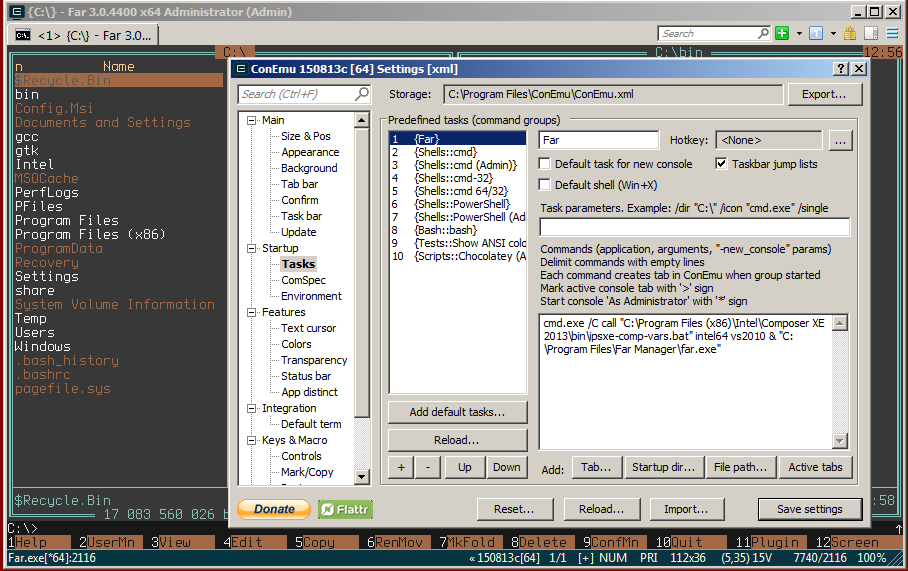
Then, all the Intel build environment commands will be run automatically every time the ConEmu terminal is started (or the task is started), so you would not need to runt it manually.
More information on the command line interface with the Intel Fortran Compiler see Using the Command Line.
13.3. Tweaking Makefile
|
|
In most cases only the model source code file(s) may need tweaking. This is defined in the variable SRC of the Makefile. Also, path to the Modelling tools, HEDTOOLSDIR, may need an update. Everything else should work out of the box. |
13.3.1. Concepts
The two most important concepts for writing Makefile are variables, macros, rules and targets. In essence, Makefile just defines rules that build targets from their prerequisites using variables and macros.
Everything that starts from # is considered a comment.
Variables are defined as in shell scripts, for example:
# This variable defines the compiler command
GF_FC = gfortran
Variable can be expanded. The simplest kind of it is just assignment of a value from another variable:
# FC now gets value from GF_FC
FC = $(GF_FC)
A variable can get value from the output of the a shell script, then it should start from shell keyword, e.g.
# Check GCC version, it just calls: gfortran -dumpversion
#  gfortran is obtained from the variable GF_FC
GFORTVERSION = $(shell $(GF_FC) -dumpversion)
There are also automatic variables, such as:
$@ The filename representing the target, $< The filename of the first prerequisite, $? The names of all prerequisites that are newer than the target, separated by spaces, $^ The filenames of all the prerequisites, separated by spaces, $* The filename of the target without suffix.
Macros are like multi-row variables that define a sequence of actions, a kind of "subroutine." For example, the following macro has the name AUTOGEN_COMMENT, it uses the standard echo shell command and file redirection > to write (autogenerate) a piece of source code, the file name is defined by $(AUTOGEN_HEADER):
# Autogenerated include file.
define AUTOGEN_COMMENT
  $(shell echo "!> @file $(AUTOGEN_HEADER)"                 > $(AUTOGEN_HEADER))
  $(shell echo "!! Autogenerated header for module RANDOM"  >> $(AUTOGEN_HEADER))
  $(shell echo "!! Sets compiler-specific code for PRNG"    >> $(AUTOGEN_HEADER))
  $(shell echo "!+---------------------------------------+" >> $(AUTOGEN_HEADER))
  $(shell echo "!| WARNING: auto-generated, do NOT edit  |" >> $(AUTOGEN_HEADER))
  $(shell echo "!+---------------------------------------+" >> $(AUTOGEN_HEADER))
endef
This sequence of actions can be called just like a variable:
$(AUTOGEN_COMMENT)
Targets define the file (e.g. executable program name) or other thing (e.g. some other target) that we are going to build. The line may also include prerequisites we need for compiling/building and finally the command(s) that actually do the build. In the simplest form a target with the name target_0 can be written like this:
target_0: prerequisite_1 prerequisite_2
    commands
Then the make system checks that prerequisite_1 and prerequisite_2 do exist and are newer than the target (by the file modification time), and then rebuilds the target_0 using commands. The system may go to other targets that are difened by the prerequisites to update them.
|
|
The commands that are defined to build a target in the Makefile (i.e. below the colon : part) must start from the TAB symbol. |
For example, the part below has the target BASE_UTILS.o (compiled object file), the prerequisite for compiling this file is Fortran source code BASE_UTILS.f90, The system builds the target BASE_UTILS.o using the compiler defined with $(FC) with compiler flags $(FFLAGS) -c, also here $< is the first prerequisite, in this case the source code file (BASE_UTILS.f90).
BASE_UTILS.o: BASE_UTILS.f90
    $(FC) $(FFLAGS) -c $<
If the system does not find the target file, it is compiled using the provided rule commands. Furthermore, if it finds out that we have already got the target file BASE_UTILS.o but it is older than the source code BASE_UTILS.f90 (the prerequisite), then this means that the target is "outdated" and should be re-compiled from the source.
A target may also be defined by a variable, e.g.
# Produce tweaked include file for PRNG
$(AUTOGEN_HEADER): $(BASE_RANDOM.f90) $(THIS_FILE)
    $(AUTOGEN_COMMENT)
    $(AUTOGEN_CODE)
The above code defines the rule to write the source include header file with the name defined by $(AUTOGEN_HEADER) with the prerequisites $(BASE_RANDOM.f90) and $(THIS_FILE) using the actions defined by the two macros (or variables): $(AUTOGEN_COMMENT) and $(AUTOGEN_CODE).
13.3.2. Basic parameters
There are only few parameters in the Makefile that may need manual tweaking. The two variables that always need tweaking are, understandably, the file name(s) for the model code: SRC and the name of the executable OUT (although the latter may always be MODEL.exe).
The variable SRC defines the main source code file(s) for the model (HEDTOOLS are separate).
# These names should be set for particular project,
# Most probably they should be edited manually for each specific project
# SRC is the name of the main source code (can be several files). Note that
#   Intel fortran doesn't like f95 file extension, use f90
# OUT is the executable file

SRC = HEDG2_03.f90

OUT = MODEL_00.exe
Several files of the model source code can be defined, e.g.
SRC = HEDG2_03.f90 HEDG2_03U1.f90 HEDG2_03U2.f90 HEDG2_03U3.f90
or wildcards for files in the current directory (or several wildcards) can be used:
SRC = HEDG2*.f90
The variable HEDTOOLSDIR defines the location of the source code for the modelling tools/modules. In most cases the file hierarchy is simple, model code and the HEDTOOLS code are in separate subdirectories.
Workdir
 |
 |-- Model1   # Directory for Model 1
 |-- Model2   # Directory for Model 2
 |
 `-- HEDTOOLS # Directory for modelling tools
      `--IEEE
In such a case, HEDTOOLSDIR is defined in the Makefile as follows:
# Path to HEDTOOLS and IEEE non-intrinsic libs
HEDTOOLSDIR = ../HEDTOOLS
IEEEPATH = $(HEDTOOLSDIR)/IEEE
Here are some of the variables that might need re-definition:
-
FC is the default compiler,
-
SRC is the source file name(s) for the model (almost always needed!),
-
OUT is the executable name to be built,
-
HOST_HPC_ROOT host name of the HPC cluster where the model is run by submitting the cluster job (normally fimm),
-
HEDTOOLSDIR path to the modelling tools (HEDTOOLS),
-
IEEEPATH path to the non-intrinsic IEEE modules (normally $(HEDTOOLSDIR)/IEEE),
-
GF_STATIC GNU compiler options for static build,
-
GF_TRAPS GNU compiler options for IEEE arithmetic traps,
-
GF_RCHECKS GNU compiler options defining runtime code checks,
-
GF_FFLAGS GNU compiler flags, optimisations etc.,
-
IF_ - Intel compiler options with the same purposes as the above GF_-flags.
The definition of the supported compilers and the the default compiler (that is used if make is called without parameters) is like this:
# Supported Fortran compiler types
GF_FC = gfortran
IF_FC = ifort
SF_FC = f95

# Choose the default compiler type
FC = $(GF_FC)
So, to tweak the Makefile to use the Intel compiler as default, just change this:
FC = $(IF_FC)
|
|
The Makefile code is documented, just read the comments and explanations for the different variables and macros. |
14. Using Microsoft Visual Studio
14.1. Working with the source code of the Modelling Tools
This is a difficult but flexible method.
Developing and debugging the code that uses the source code of the HEDTOOLS modelling tools with Microsoft Visual Studio on the Windows platform should follow such a workflow.
-
Create the model project in Microsoft Visual Studio as usual.
-
Include the source .f90 files from HEDTOOLS that are used in the project into the current Microsoft Studio project. Source files can be just copied into the model source code directory for convenience.
-
Manually tweak the source code for these non-portable modules, that make use of auto-generated include files in the make system. Currently, there are two such modules: BASE_RANDOM and IEEE Modules
-
Compile/Build/Debug and work with the model code(s) as normal from within the Misrosoft Studio
-
The model code can be (re)built using the command line tools and the make-based system. Just do not forget to point to the location of the original unedited HEADTOOLS code within the Makefile. The Modelling tools code tweaked manually as a part of the Visual Studio Project cannot be used by the make system.
14.2. Building the Modelling Tools as a static library
This is the easiest method not requiring any manual tweaks.
An easier and more convenient way to include the HEDTOOLS modelling tools
to a Microsoft Visual Studio / Intel Parallel Studio Project is to build
the tools as a static library that is then included
into the current model coding project. This method does not require manual
tweaking of the modelling tools source code and takes full advantage of the
automatic make system
[Although, if IEEE Modules are
used in the code, the code should be tweaked manually]
. Also, the same library
file can be included into many different Visual Studio projects. However,
the tools library must be built using exactly the same platform and compiler.
|
|
Never mix static library produced with GNU fortran into Intel Parallel Studio projects or vice versa, or even different versions of Intel Parallel Studio Fortran—the library and the project code must be built using the same compiler. |
First, build the HEDTOOLS modelling tools as a static library using the make system with FC=ifort, this is the default make target. Do not forget to make sure the Intel Parallel Studio Command Prompt Environment has been correctly prepared prior to the build process.
make FC=ifort
On the Windows platform with Intel Fortran compiler, this will produce a static library file with this name: lib_hedutils.lib as well as many .mod header files. For convenience, the make system also produces a zip archive containing all the re-distributable tool files.
|
|
The Makefile producing the library requires two command line GNU utilities: uname and zip. Windows versions are available from Cygwin and other distributions. If these utilities are not available, the static library is still produced although the handy zip file distribution is not generated. |
|
|
Binary pre-built HEDTOOLS library ready to be included into other projects is available at the DOWNLOADS section. This distribution is built with the Intel Fortran ifort version used currently at TEG. The compiler version used to build the HEDTOOLS library should agree with the version used for the project. To check the version call ifort program without parameters in the Windows terminal (command prompt window). |
14.2.1. Include HEDTOOLS into Microsoft Visual Studio project
Once the HEDTOOLS library distribution is available, either custom built as above or downloaded from the pre-built distribution site, it can be included into a Microsoft Studio project.
|
|
Make sure the project is built for the 64 bit platform (x64) if the HEDTOOLS library is built as x64. They should always be the same! Set the correct target platform in the project Properties. The pre-built distributions at DOWNLOADS are 64 bit. Note that the error message issued by the compiler if the target platform does not match is not intuitive ("modules built for a different compiler version"). |
First, copy .mod files to the current Visual Studio Project folder containing the source code .f90 files. The library itself should be also placed there. It is convenient to just unzip the whole content of the redistributable zip file created by the make system.
Then, insert the lib_hedutils.lib static library file into the project, use the menu Add → Existing Item menu.
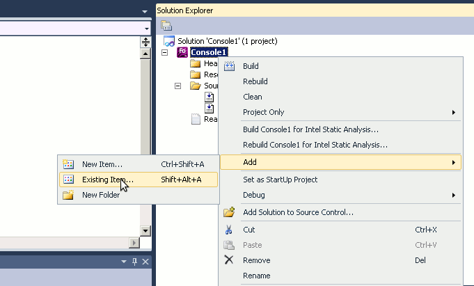
It is also possible to add the library into the project directly from the HEDTOOLS directory, in such case, also add all the .mod from HEDTOOLS to the project. Then, the library and .mod files are accessed directly from the Modelling Tools folder and should not be copied to the current project folder and can be included from their own directory to several Visual Studio projects.
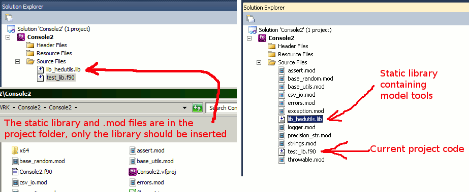
Now the code should build successfully (calling the modelling tools code from the library) as normal (e.g. Build → Build Solution).
14.2.2. Link error: LNK2005
There may be a LNK2005 problem with the LIBCMTD.lib library:
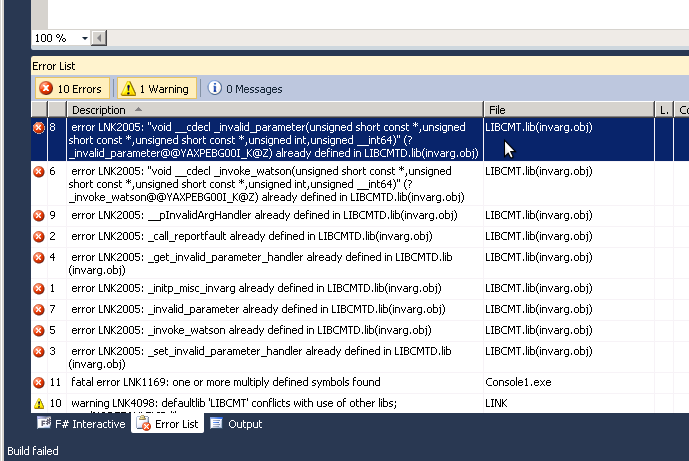
It is also possible that the Microsoft linker issues another LNK2005 error, related to double definition of symbols in libifcoremdd.dll.
In such a case, go to Properties → Fortran → Libraries and select non-DLL Runtime Library, e.g. Debug Multithreaded instead of Debug Multithreaded DLL:
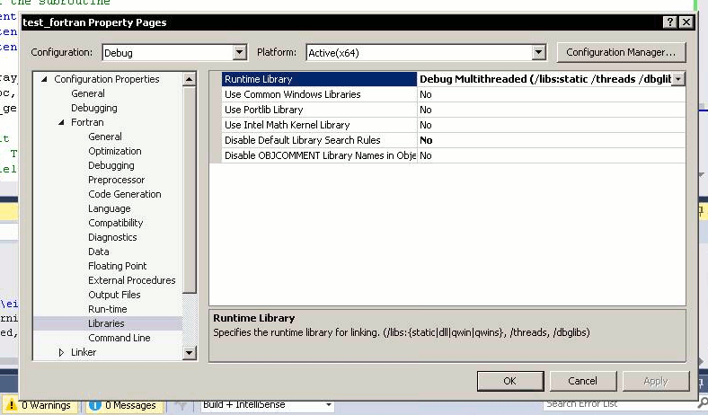
and Multithreaded instead of Multithreaded DLL:
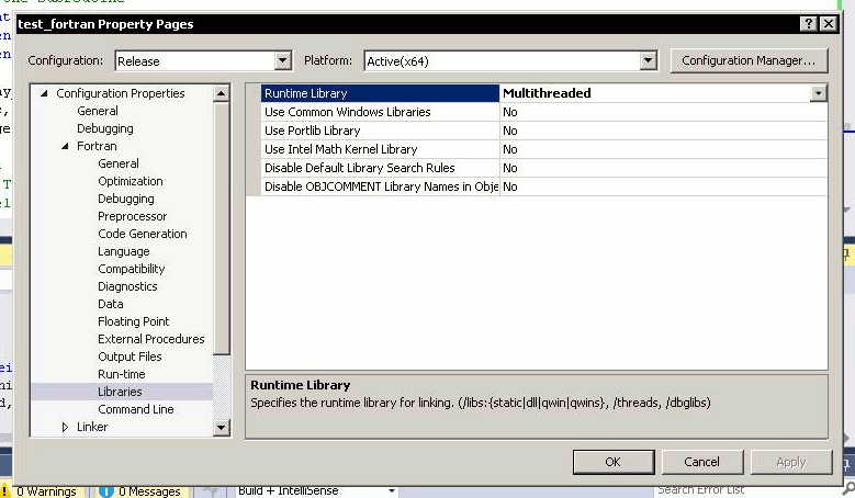
This must solve the issue by forcing linking with the static runtime library.
If, however, linking with DLL is necessary for any reason, or the LNK2005 problem persists, go to Properties → Linker → Input and insert the problem library libcmtd.lib to the Ignore Specific Library field:
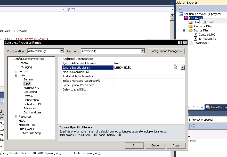
It might also help placing libifcoremdd.lib into the ignore list as above: Properties → Linker → Input then Ignore Specific Library.
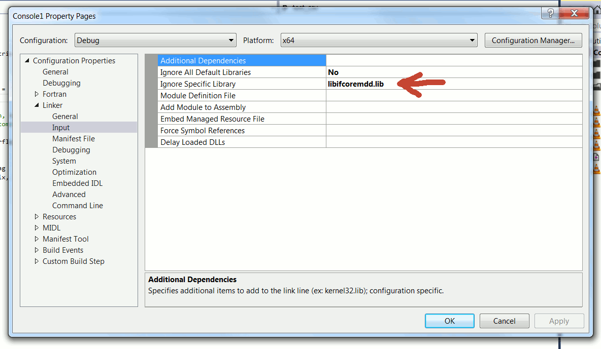
The LNK2005 problems could potential occur with the following libraries (both single- and multi-threaded versions are included):
-
libifcore.lib
-
libifcoremt.lib
-
libifcoremt.lib
-
libifcorertd.lib (libifcorertd.dll)
-
libifcoremd.lib (libifcoremd.dll)
-
libcmtd.lib
-
libcmt.lib
-
libcmtd.lib
-
msvcrt.lib (msvcrt.dll)
-
msvcrt.lib (msvcrt.dll)
-
msvcrt.lib (msvcrt.dll)
The main solution is to use non-DLL runtime library. Otherwise, it might be worth to include the respective .lib file into the ignore list as above.
From now, it should (hopefully) build without further issues. The modelling tools are now automatically inserted by the compiler into the executable code from the static library provided as if the subroutines and functions were intrinsic.
14.2.3. Using the static library tools for command line building
Finally, if you like to build code with the static library from the command prompt rather than Visual Studio IDE, it is also easy:
ifort file.f90 lib_hedutils.lib
This command compiles and links the code in file.f90 with the library.
The static library can be built on any of the supported platforms (Windows, Linux, Mac) and compilers (e.g. GNU gfortra and Intel Fortran). But note that on Unix systems and GNU gfortran on Windows the library has an .a rather than .lib file extension. The redistributable zip file that is produced when building the library contains a small Readme.txt file.
15. Using Code::Blocks IDE
15.1. Building the Modelling Tools as a static library
Working with the Code::Blocks IDE is similar to that with Microsoft Studio. The simplest way to get it running is to (1) build HEDTOOLS as a static library using the make system, (2) copy the library file lib_hedutils.a (or lib_hedutils.lib) and all the .mod files produced by the make build system into the working project directory, add the library file to the project file using the Project → Add Files menu. After this it should build within the IDE.
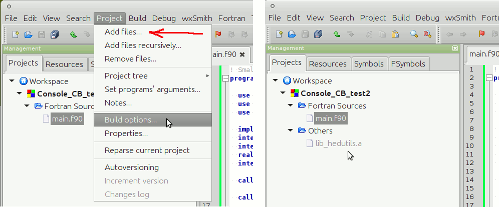
When building, a link order issue may appear, but this does not affect anything, so in most cases just ignore it.
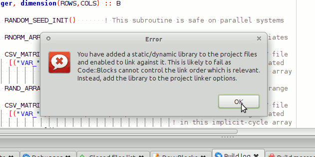
Alternatively, the library can be inserted using the Project → Build Options → Linker settings. Using this method, you might get an issue with the compiler not being able to find the library (as it is not in the LIBPATH). Not keeping relative path to the library will solve the problem.
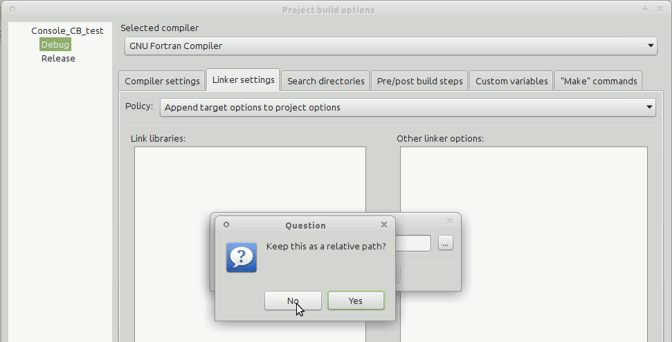
15.2. Using the custom Makefile
Another method to use the HEDTOOLS bundle in Code::Blocks IDE is to set up the program build directly from the custom Makefile: Project → Properties
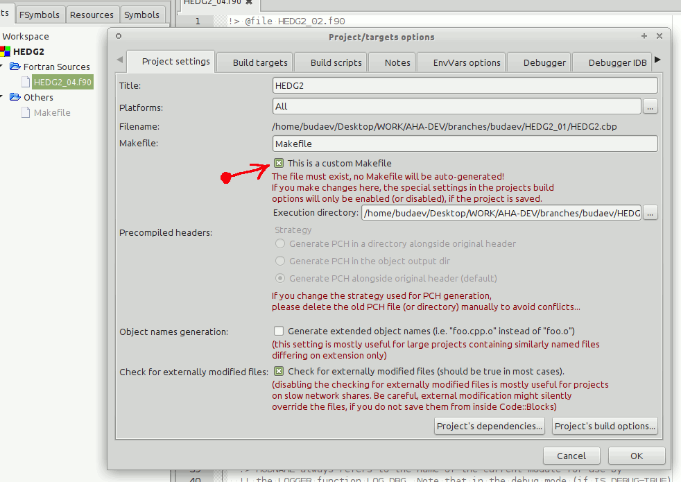
and setting target paths as in the Makefile, i.e. in the "." directory (rather than the default \bin). Also, the Makefile commands for Debug (Project → Build options) should include the DEBUG=1 flag (see the GNU Makefile command line options for debugging).
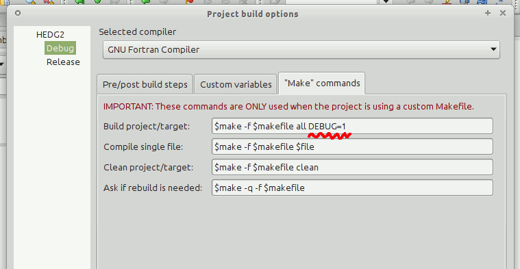
This is the most universal and flexible method that uses the same Makefile for building both on the command line and from the IDE.
|
|
A Code::Blocks project template for the AHA Model is available
in the ^/trunk/scripts folder on the Subversion repository:
Project.cbp.
This file should be copied to the project folder. the svn command for
this is: svn export https://tegsvn.uib.no/svn/tegsvn/trunk/scripts/Project.cbp |
16. Manual builds of HEDTOOLS
16.1. Editing source codes
If the model is built without using the automatic GNU make utility and the supplied Makefile, you should take care about the dependencies and header files yourself. These are the modules that require manual source tweaking in such cases:
These pieces of code should be edited manually depending on the compiler and its version used. Please check your documentation. Make sure all source code files for the model as well as for the HEDTOOLS are included in the project. Many IDEs allow generating (importing) project from a supplied Makefile and recognize GNU make format. This could make work a little easier.
16.2. Using static library
Another option is (1) to build the modelling tools as a static library using the make system. (2) Compile the model and link the tools in from the library. Then, no manual edits may be required. Refer to the Readme.txt file that is produced with the static library. When using the Intel Fortran compiler on Windows, make sure the command prompt environment is correstly set up.
# (1) in the modelling tools directory
HEDTOOLS]$ make             # make the static library of the Modelling Tools
...
# (2) in the model code directory (make sure .mod and library files are placed there)
#     compile model code link with the library producing the executable
test_library]$ gfortran test_lib.f90 lib_hedutils.a
This is a small test program code producing two random matrices and saving them to CSV:
! test_lib.f90 :: Small test of the HEDTOOLS
program test_library

  use CSV_IO        ! we use these modules
  use BASE_UTILS    !   from HEDTOOLS
  use BASE_RANDOM

  implicit none
  integer, parameter :: ROWS=1000,  COLS=20
  integer :: i
  real, dimension(ROWS,COLS)    :: A
  integer, dimension(ROWS,COLS) :: B

  call RANDOM_SEED_INIT()        ! This subroutine is safe on parallel systems

  call RNORM_ARRAY(A)            ! Generate a matrix of random normal variates

  call CSV_MATRIX_WRITE(A, "file_matrix_a.csv",& ! Save the matrix to CSV file
        [("VAR_" // TOSTR(i,COLS),i=1,COLS)])    ! Column names are generated
                                                 ! in this implicit-loop array

  call RAND_ARRAY(B,10,100)      ! Generate a random integer matrix with range

  call CSV_MATRIX_WRITE(B, "file_matrix_b.csv",& ! Save the matrix to CSV file
        [("VAR_" // TOSTR(i,COLS),i=1,COLS)])    ! Column names are generated
                                                 ! in this implicit-loop array
end program test_library
17. Plotting tools
There are a few plotting tools in the HEDTOOLS/tools directory. They are non-essential and implemented separately from the main HEDTOOLS code, although do use HEDTOOLS code procedures. This is done to keep the dependencies to the absolute minimum.
|
|
As from r9339, plotting tools migrated from PGPLOT to DISLIN due to better DISLIN support on Microsoft Windows and the change of the licensing policy of GrWin library (license key needed, free use license key is now time limited). Both PGPLOT and DISLIN versions of the tools are now supplied in two separate directories: gtools.pgplot and gtools.dislin. |
17.1. DISLIN
The DISLIN is a powerful cross-platform graphics library that can be called from Fortran, C/C++ and other programming languages. For more information refer the web page: http://www.dislin.de/.
DISLIN is developed in the Max Planck Institute for Solar System Research.
17.2. PGPLOT
Currently they make use the PGPLOT Fortran plotting library, but the plotting part is quite small and simple, so they can be easily recoded to use a different toolbox for plotting (e.g. PlPlot or DISTLIN). PGPLOT is chosen because it is very small, simple to use and can be built for Linux (and various Unix clones) and Windows. PGPLOT in included in the standard Ubuntu Linux repositories. For Windows, PGPLOT is a part of the GrWin library.
Plotting tools should be built separately from HEDTOOLS and the model code and then placed to some directory in the PATH so the system is able to find the executables. They should be called from the main model code using the standard intrinsic Fortran procedures to run the system (shell) commands: execute_command_line or (older system).
17.3. Build
To build the plotting tools using the default parameters issue this command in the main HEDTOOLS directory:
make tools
17.4. Calling plotting utils from Fortran code
Here is an example of calling the scatterplot utility using a wrapper (call_external) to the intrinsic execute_command_line subroutine.
!> The name of the **scatterplot** program (htscatter.f90 from HEDTOOLS)
!! executable.
character(len=*), parameter, public :: EXEC_SCATTERPLOT = "htscatter.exe"
...
...
!> Call external command to plot the data scatterplot.
call call_external(                                                       &
      command = EXEC_SCATTERPLOT // " " // csv_file_here // " " //        &
                                           csv_file_here // PS,           &
      suppress_output = .TRUE., suppress_error = .TRUE.,                  &
      is_background_task = do_background )
17.5. List of utilities
-
hthist.f90 — histogram of data saved in a CSV file, any column can be plotted.
hthist 2 data_file_csv plot_file.png
-
htintrpl.f90 — linear and non-linear interpolation of data provided on the command line. Example:
htintrpl.exe [1 2 3 4] [10., 45., 14., 10.] [2.5 1.9] [linear] [file.ps]
-
htscatter.f90 — scatterplot of data saved in a CSV file. Example:
htscatter data_file_csv plot_file.png
17.6. Notes on PGPLOT Windows (GrWin)
Building with GrWin + PGPLOT. On the Microsoft Windows platform, depending on the directory location of the GrWin library (it is different on 32 and 64 bit versions of Windows), one may need to change the GRWIN_ROOT value in the tools own Makefile that is located in HEDTOOLS/tools:
# Root directory of the GrWin installation on Windows.
# NOTE: can differ in 32 and 64 bit distributions!
GRWIN_ROOT = C:/GrWin/MinGW_gfortra
It is possible to build the Microsoft Windows executables of the plotting
utilities on a machine with the GrWin library installed and run on another
machine without these libraries. However, the GrWin graphics server will
be unavailable on the later machine and the interactive graphics display
window could not be opened. Therefore, only saving the plot to a PostScript
output file will work
[This is what is needed as we do not (normally)
display plots on the screen.]
.
There is an additional possible caveat: (a) there should be the PGPLOT main
font file grfont.dat installed somewhere on the system
[If the
font file is not found the system will issue this error: PGPLOT, Unable to
read font file: grfont.dat]
and (b) the PGPLOT_FONT environment variable
[It can be set in the Windows Control Panel.]
must indicate the
path where it is located. A quick and dirty method to make the graphics
working is just to to copy the font file into the current directory.
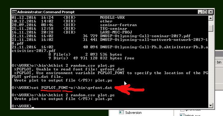
18. Using IaaS workstation: AHA_Workshop
18.1. Linux-based Workstation
The University of Bergen provides a cloud-based Infrastructure as a Service (IaaS) system based on OpenStack. There is a virtual workstation for developing the AHA Model based on this cloud infrastructure. The "virtual developer 's computer" has the Debian Linux OS and has all the essential software pre-installed and ready for use out of the box.
|
|
The current system is based on GNU gfortran and Code::Blocks IDE. This is open source software under the GNU license. Intel Fortran and any other proprietary software can be installed individually provided there is valid license. |
18.1.1. Connecting the cloud workstation
To connect the cloud-based AHA Workshop you need the X2Go client software installed on the local physical computer that is used to access the cloud workstation. Once connected, it works just like a physical Linux computer preloaded with all the required software:
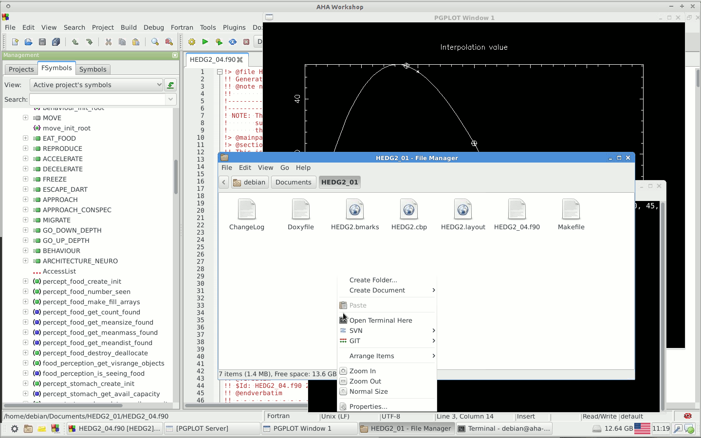
There is even less difference from the look and feel of a physical system if the remote access X2Go client is working in the full screen mode.
X2Go Client can be downloaded for Windows from the official website: http://wiki.x2go.org/doku.php/start .
On the Ubuntu Linux installation is trivial from the command line:
sudo apt-get install x2goclient
The access is based on ssh key file. You can supply your own ssh public key or get a private secret ssh key (xxx.pem) from the administrator.
|
|
If you have got an ssh key file (.pem), it should be kept secret in a secure place not accessible for anyone else. This key file is the only method to get access to the cloud AHA Workshop workstation (there is no password). The graphical connection session is tunnelled via ssh and is secure. |
The user name at the AHA Workshop workstation is debian. To connect, you will also be given an unique ip address. The session type for the Linux machine is always XFCE. Xfce is a simple and lightweight desktop environment. Check out its official web site: https://www.xfce.org/ and the Getting Started guide.
A typical configuration of the AHA Workshop connection is like this:
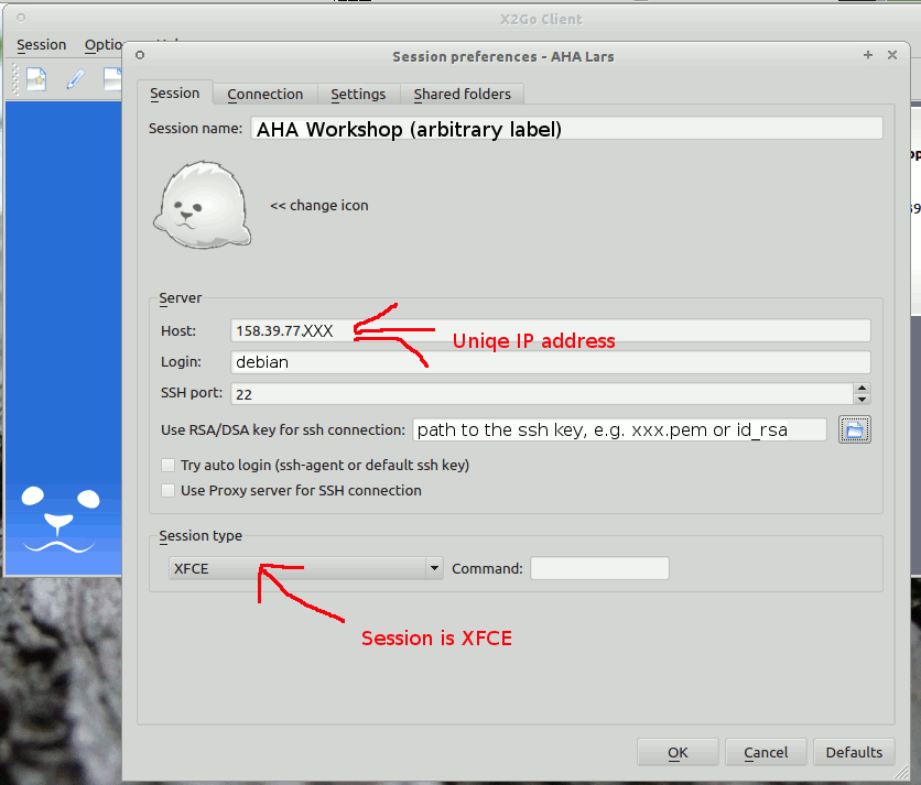
You may also like to set up the screen resolution in the Settings tab. There is also a useful tab for setting the Shared folders: you can automatically mount your local folder into the remote system. It is then easy to transfer data to and from the local to the cloud machine. Do not forget to tick "automatically mount" here. The mounted remote folders are under /home/debian/media/disk/:
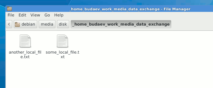
If the local system has a high resolution display, the AHA Workshop virtual PC may have huge fonts (that looks as if everything just in zoom-in). In such a case one has to adjust the screen DPI: Go to Settings tab and set Set display DPI to 100 or a higher value if your display is in HD mode (default DPI is 96).
It also makes sense to disable the remote sound support in the Settings tab as it could reduce CPU load on the local machine and avoid any sound errors. There is no sound on the AHA Workshop cloud PC anyway.
In addition to the full graphical connection mode, it is also possible to connect the remote system via plain ssh (using the Terminal):
ssh debian@ip_address
18.1.2. Initial setup: Subversion and IDE Project
Subversion command line client is installed here. To get your Subversion files in the Documents folder double-click Home to open the file manager, then Documents, right click and select Open Terminal here. When the Terminal window opens issue this command:
svn --username user_name checkout https://tegsvn.uib.no/svn/tegsvn/_your_svn_path
It will also ask your svn password on the first run, use option to save it. Good to save to avoid retyping the password on any svn operation.
This can also be done using the SVN client integrated into
the default Thunar file manager: go to Documents, right-click and select
Create Folder, enter the name of this new folder
[Caveat: the
built-in svn client does checkout into an existing folder.]
, it will then
contain the code. Second, go into the new folder, right-click, select SVN
then Checkout:
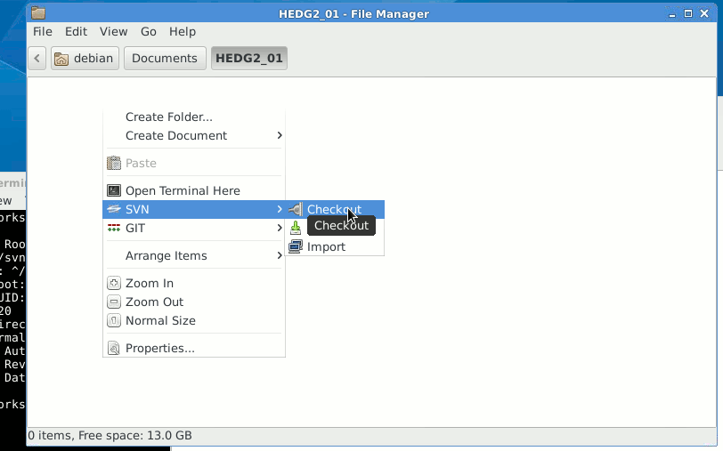
and finally put the SVN branch URL into the opening window.
Code:Blocks. It is also easy to get an initial Code::Blocks IDE Project file template linked with the Makefile. Go to the working copy containing the code, open Terminal and issue:
svn export https://tegsvn.uib.no/svn/tegsvn/trunk/scripts/Project.cbp
|
|
Configuring the project template file is only necessary if the Makefile is used for building the project. The Project.cbp file is configured to use the existing Makefile in the current directory. If the existing Makefile is not used, Code:Blocks project should be configured from scratch, as needed. |
The same using the file manager: go to the working directory containing the model code, right-click and select SVN then Export, and then put the Code:Blocks Project file path (https://tegsvn.uib.no/svn/tegsvn/trunk/scripts/Project.cbp).
Then you can open this project file from the Code:Blocks IDE. The first thing to do here is (1) delete the fake Fortran file some_file.f90 from the Workspace pane and (2) Open valid Fortran source code files (can be easily done by drag and drop), right click the file tab and select Add to active project:
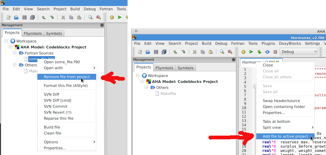
To complete the Code:Blocks project configuration, set the correct executable
name that is generated into the build options. The executable name should
coincide with that in the Makefile: variable $(OUT)
[It is
defined as OUT=executable_name.exe in the Makefile.]
. Go to the menu
Project, then Project options and switch to the Build targets tab:
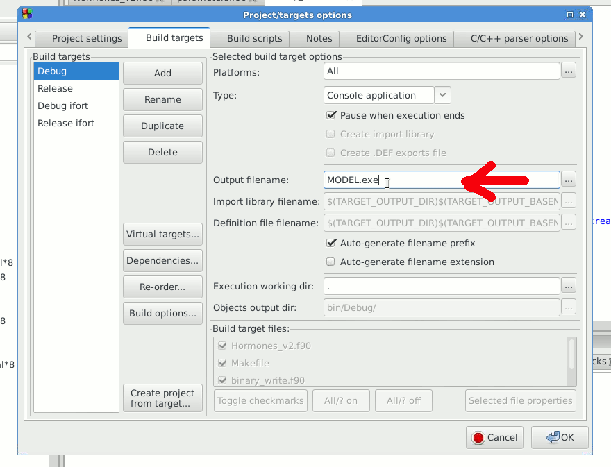
18.1.3. Notes on the tools
The Code::Blocks installation on the AHA Workshop machines has a simple Subversion menu integrated into the tools menu. This allows to run basic elementary commands like update, diff, commit and revert.
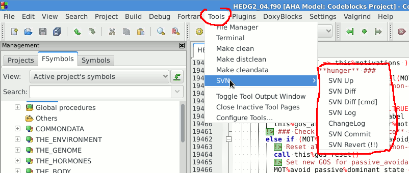
For example, commit calls an entry field for the commit message:
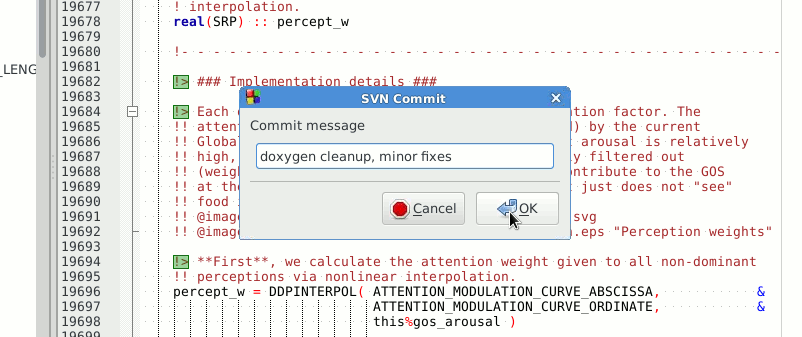
The Xfce Thunar file manager has a useful feature allowing to configure custom commands and actions on files and folders. For this click Edit, then Configure custom actions. For example, it is easy to make a right-click menu entry to check the differences between the working file and the SVN server version (i.e. do svn diff using a graphical program, e.g. meld).
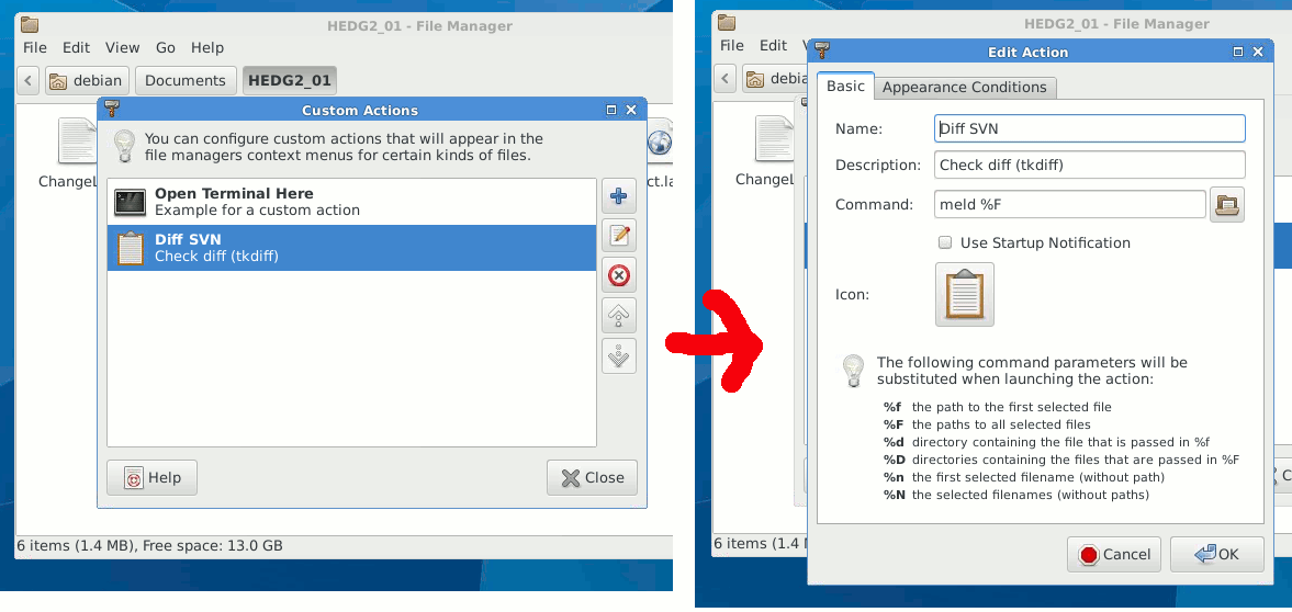
Then right clicking on a file will also bring a menu entry to check the difference between the local and SVN versions:
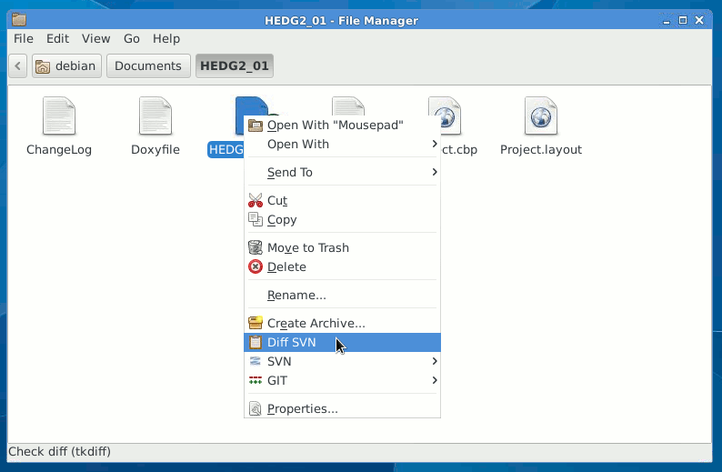
Similarly, one can configure menu items for performing other actions, for example the make and make distclean:
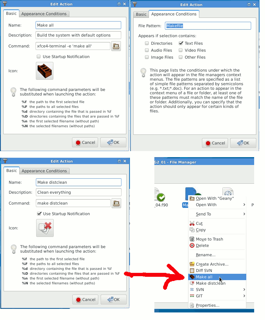
Note that a better command for pasting into the Make is this long:
xfce4-terminal -x bash -c "time make ; echo BUILD DONE, ENTER to CLOSE ; read"
It does not close the terminal upon completion and also shows how long it took to do the build (the time command is used for this).
18.1.4. System maintenance
The cloud PC should be kept in secure condition by regular software updates. This is done easily from the terminal using this command:
sudo apt-get update && sudo apt-get upgrade
The Linux package system might sometimes keep downloaded updates and dependency components that no longer required. To clean these dependencies issue this command in the terminal:
sudo apt-get clean && sudo apt-get autoremove
Installing additional software can be done using the synaptic GUI system:
sudo synaptic
Or on the command line from the terminal. For example, to install the R base package issue this:
sudo apt-get install r-base
For more details check the Debian Linux documentation site: https://www.debian.org/doc/user-manuals